In the spirit of looking at fancy word topics, this post is about variational inference. Suppose you granted me one super power and I chose the ability to sample from any distribution in a fast and accurate way. Now, you might think that’s a crappy super-power, but that basically enables me to fit any model I want and provide uncertainty estimates.
To make the problem concrete, lets suppose you are trying to sample from a distribution \(p(x)\). To make matters worse, you only know \(f(x) = Cp(x)\) up to some constant \(C>0\). Well that seems a little contrived, right? But let’s say I use the following Bayesian linear model (see here for an introduction): \[ \begin{aligned} y | \beta &\sim \text{Laplace}(X\beta, 1)\\ \beta &\sim N(0,1). \end{aligned} \] I can calculate the posterior up to constants quite easily by Bayes rule: \[ p(\beta | y, X) \propto p(y | X, \beta)p(\beta | X) = \frac{1}{2}e^{-\sum_{i=1}^n|y_i - (X\beta)_i|}\frac{1}{\sqrt{2\pi}}e^{-\frac{1}{2}\beta^T\beta}. \] Looks easy enough, but trying to integrate the above function (over \(\beta\)) using trapezium rule in \(100\) dimensions is pretty difficult.
Generally there are two approaches to sampling \(p(x)\). One is Markov chain Monte Carlo which is what packages like Stan do. Instead today we are going to look at approximating \(p(x)\), which is called variational inference. The general goal is to have an easy to sample distributions with densities \(q_\lambda(x)\) indexed by some parameters \(\lambda\), and pick the best \(\lambda^*\) so that \(q_{\lambda^*}(x) \approx p(x)\). So now the natural question is, how do we measure the approximation accuracy of \(q_\lambda\)?
Kullback - Leibler divergence
Suppose you’ve outsourced your sampling needs to a dodgy sampling company ran by me. You want to sample some \(N(0,1)\) random variables, but unfortunately I only have Laplace\((0, 2^{-1/2})\) random variables (which has the same mean and variance as the normal). I send you these anyway and tell you they are normally distributed in an attempt to fool you.

Our national sport, fooling people
After a while you notice that my samples have a lot of outliers. That’s because the Laplace distribution has heavier tails. So you plot out what you got from me against a normal density and see this:
library(rmutil)
tibble(received = rlaplace(n=100, s=1/sqrt(2))) %>%
  ggplot(aes(received)) +
  geom_histogram(aes(y=..density..), bins = 20) +
  stat_function(fun = dnorm, args=list(mean=0, sd=1), colour='red') +
  labs(x='', y='Density')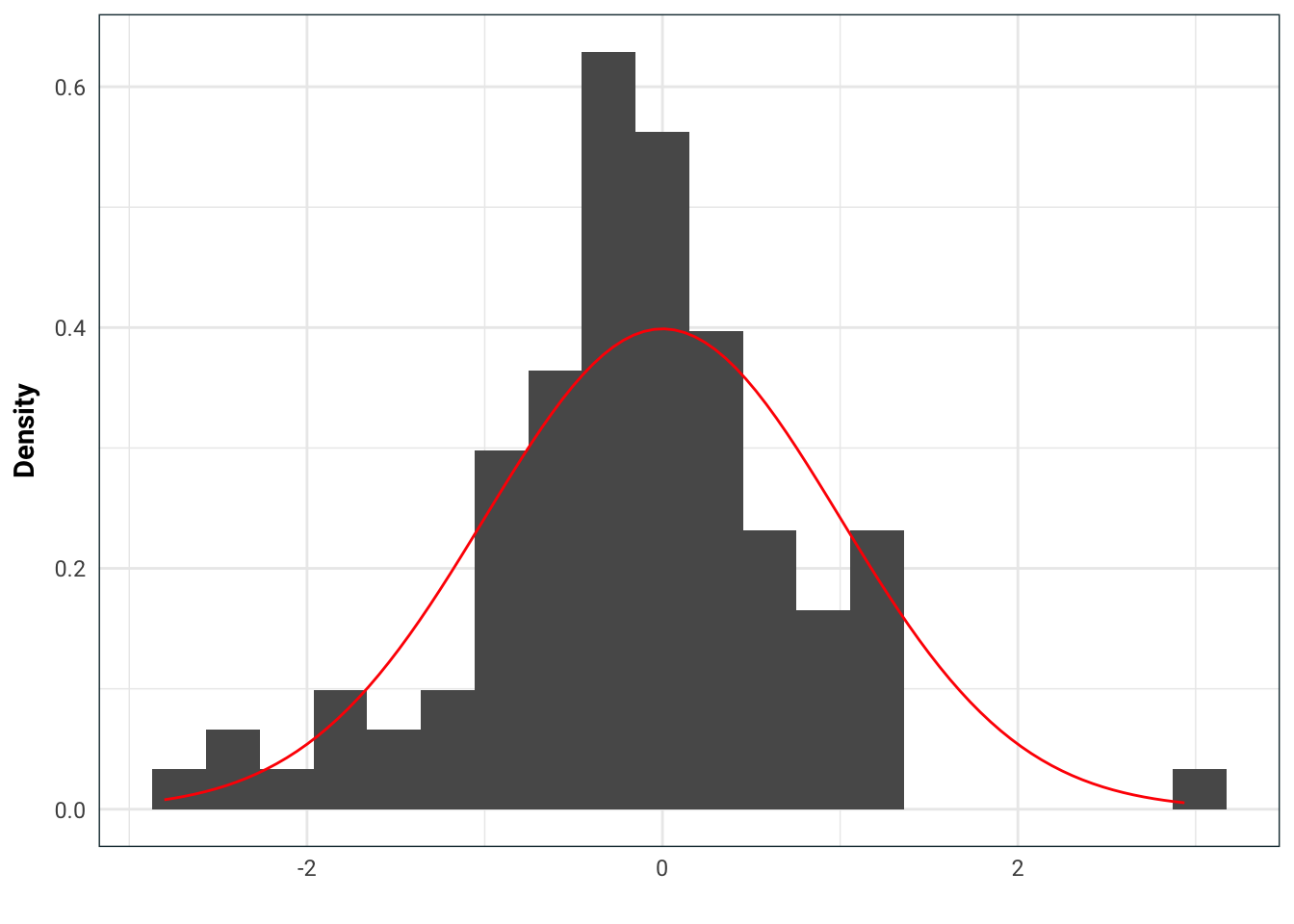
You notice that it looks awfully like I’m sending you Laplace distribution samples but before you go to your boss, you want some hard statistical proof of this trickery. So you do a likelihood ratio test to test \(H_0\): the samples come from a \(N(0,1)\) distribution vs \(H_1\): the samples come from a Laplace\((0, 2^{-1/2})\) distribution. This is a classical hypothesis test, take \[ L = \log\left(\prod_{i=1}^n \frac{q(x_i)}{p(x_i)}\right) = \sum_{i=1}^n \log\left(\frac{q(x_i)}{p(x_i)}\right), \] where \(p\) is a normal density and \(q\) is a Laplace density, and reject the null hypothesis if \(L > c\) for some threshold \(c\). So with my dodgy samples, the value of \(L\) you get is
samples <- rlaplace(n=100, s=1/sqrt(2))
L <-  prod(dlaplace(samples, 0, 1/sqrt(2)) / dnorm(samples, 0, 1)) %>% log
print(L)
#> [1] 10.33139So it seems pretty likely that I’m tricking you and you go to your boss and complain.

Notice that this testing isn’t symmetric. Suppose the roles of the normal and Laplace distributions were reversed, i.e. I am giving you normal distribution samples, where as you wanted Laplace. What would the test say then?
samples <- rnorm(n=100)
L <-  prod(dnorm(samples, 0, 1) / dlaplace(samples, 0, 1/sqrt(2))) %>% log
print(L)
#> [1] 0.5965472Well now the number we get is lower than before? This makes sense when you think about it. If give you Laplace and you expect normal, there is going to be a lot of samples that have very low probability of appearing. When the roles are reversed and I’m giving you normal distribution when you expect Laplace, then you expect the tails to have more samples but they don’t come. The latter event has a much higher probability than the former event.
So your boss calls me up and tells me about your test then complains to me about the samples you received (I gave you Laplace when you wanted normal). I grudgingly admit I have been tricking you but promise to resolve the issue.

No more tricks please
Unfortunately, normal samplers are hard to come by and expensive, so I go back to my old tricks, but now I know I’m being watched. I go out shopping for other distribution samplers that are cheaper. Since I know you are doing a likelihood test, I know that if I send you samples from distribution with density \(q\), your test statistic will be (at least asymptotically) \[ \text{KL}(q||p) = \int q(x) \log\left(\frac{q(x)}{p(x)}\right) \, dx. \] which is the Kullback-Leibler divergence. So in my shopping, what I should do is try to minimise the Kullback-Leibler divergence.
ELBO: Evidence lower bound
Back to the variational inference, now we know we would like to select \[ \lambda^* = \text{argmin}_\lambda \text{KL}(q_\lambda||p) \] but we only know \(p(x)\) up to some multiplicative constant, \(p(x) = Cf(x)\). Well let’s start by writing out the KL divergence: \[ \begin{aligned} \text{KL}(q_\lambda||p) &= \int q_\lambda(x) \log\left(\frac{q_\lambda(x)}{p(x)}\right) \, dx.\\ &=\int q_\lambda(x) \log q_\lambda(x) \, dx - \int q_\lambda(x) \log p(x) \, dx \\ &= \int q_\lambda(x) \log q_\lambda(x) \, dx - \int q_\lambda(x) \log f(x) \, dx + \log(C). \end{aligned} \] So minimising the KL divergence is equivalent to maximising the evidence lower bound (ELBO) given by \[ \text{ELBO}(q_\lambda || f) = -\int q_\lambda(x) \log q_\lambda(x) \, dx + \int q_\lambda(x) \log f(x) \, dx. \] Why is this easier? Well remember that we can easily sample from the distribution, \(X^{(\lambda)}\), whose density is \(q_\lambda\). So and easy way of doing the integral above is to get i.i.d. samples \(x^{(\lambda)}_1, ..., x^{(\lambda)}_n\) of \(X^{(\lambda)}\) and then approximate ELBO by \[ \text{ELBO-approx}(q_\lambda || f) = -\frac{1}{n}\sum_{i=1}^n \log q_\lambda(x_i^{(\lambda)}) + \frac{1}{n}\sum_{i=1}^n \log f(x_i^{(\lambda)}). \] We can then numerically minimise ELBO-approx to find the optimal \(\lambda\).

Here comes the ELBO
So let’s go back to the early example and do it in one dimension: \[ f(\beta) = e^{-\sum_{i=1}^n|y_i - x_i\beta| -\frac{1}{2}\beta^2} \] where the \(x\) and \(y\) are given. We will simply generate these randomly, because, why not. As our approximating distribution, let’s take \(N(\mu, \sigma^2)\). Using the normal distribution has the added benefit that we can just simulate one set of \(N(0,1)\) variables \(Z_1\), …, \(Z_n\) and then scale them \(\mu + \sigma Z_i\) to get \(N(\mu, \sigma)\) variables.
y <- rnorm(100)
x <- rnorm(100)
f <- function(beta) {
  exp(-sum(abs(y - x * beta)) - .5 * beta^2)
}
z <- rnorm(500)
elbo_approx <- function(mu, sigma, z) {
  if(max(sigma <= 0)){
    Inf
  } else{
    mean( log(dnorm(mu + sigma * z, mu, sigma)) - log(f(mu + sigma * z)) )
  }
}
lambda_min <- optim(c(0, 1), function(x) elbo_approx(x[1], x[2], z))
print(lambda_min)
#> $par
#> [1] -0.09681142 0.05594696
#>
#> $value
#> [1] 378.2323
#>
#> $counts
#> function gradient
#> 83 NA
#>
#> $convergence
#> [1] 0
#>
#> $message
#> NULLWe can see that the normal distribution doesn’t approximate this distribution too well because the minimal KL divergence is still quite high. Since this is one dimensional, we can integrate the function numerically and see visually how the fit is.
int_f <- integrate(function(x) map_dbl(x, f), -Inf, Inf)
p <- function(beta) map_dbl(beta, f) / int_f$value
ggplot(tibble(x = seq(-1, 1, .1)), aes(x)) +
  stat_function(fun = p, aes(colour='Given distribution')) +
  stat_function(fun = dnorm, args = list(mean=lambda_min$par[1], sd=lambda_min$par[2]), aes(colour='Aproximation')) +
  labs(colour='',
       title='Variational inference using normal distribution',
       x='', y='Density')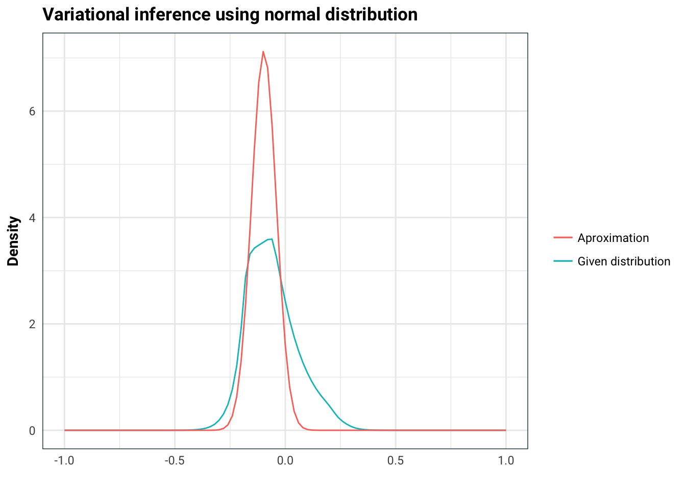
Some tools
If you want to do variational inference seriously, there are several tools available: Stan, PyMC3 and Edward to name a few. The latter two are python projects which use Theano and Tensorflow as back-ends respectively. Here is an example of the above problem Edward.
from edward.models import *
import edward as ed
import tensorflow as tf
import numpy as np
import pandas as pd
# Make up some data
n, p = 100, 5
p=5
beta = np.array([0] * p)
X = np.random.normal(size=[n, p]).astype(np.float32)
y_obs = np.matmul(X, beta) + np.random.normal(size=n)
# Edward model
beta = Normal(tf.zeros(p), tf.ones(p))
y = Laplace(ed.dot(X, beta), tf.ones(n))
qbeta = Normal(tf.Variable(tf.zeros(p)), tf.Variable(tf.ones(p)))
inference = ed.KLqp({beta: qbeta}, data={y: y_obs})
#> /Users/bati/anaconda3/lib/python3.6/site-packages/edward/util/random_variables.py:52: FutureWarning: Conversion of the second argument of issubdtype from `float` to `np.floating` is deprecated. In future, it will be treated as `np.float64 == np.dtype(float).type`.
#> not np.issubdtype(value.dtype, np.float) and \inference.run()#>
1000/1000 [100%] ██████████████████████████████ Elapsed: 1s | Loss: 156.488sess = ed.get_session()
print('Mean: %s' % sess.run(qbeta.mean()))#> Mean: [ 0.17253913 0.1097104 0.08593578 -0.01670811 -0.01817157]print('Sdev: %s' % sess.run(qbeta.stddev()))#> Sdev: [0.05179016 0.063154 0.14621048 0.08485013 0.12385876]