Bayesian statistics is an interpretation of statistics. It is used to help explain the frequentist methods and can give much more information. Even if you have never really learnt about Bayesian statistics, I guarantee you have encountered it in some way.

Bayes, it’s everywhere
In this post, we will only consider a linear model: \(y = \beta x + \epsilon\) where \(\epsilon\) is a standard normal. Suppose we have gathered some data \((Y=\{y_i\}_{i=1}^n, X=\{\{x_{k,i}\}_{k=1}^p\}_{i=1}^n)\), which consist of \(p\) predictors and \(n\) observations, and we wish to fit a linear model. There are two ways we might do this:
- Minimise the loss function \((Y - X\beta)^T(Y - X\beta)\),
- Take the \(\beta\) that maximises the likelihood of observing the observations we have, since we know \(Y=\{y_i\}_{i=1}^n\) are i.i.d. normally distributed with mean \(X\beta\) and variance \(1\).
It turns out that both approaches yield the estimate \(\hat \beta = (X^TX)^{-1}X^T Y\). Let us examine the second approach a bit more closely. Since \(Y\) is normally distributed, we can write the density function of our observations: \[ \prod_{i=1}^n \frac{1}{\sqrt{2\pi}} e^{-\frac{1}{2}(y_i - (X\beta)_i)^2}. \] Maximizing this is equivalent to minimising \(-\log(.)\) of the above, which is much more tractable, \[ \frac{1}{2}\log(2\pi) + \frac{1}{2}\sum_{i=1}^n (y_i - (X\beta)_i)^2 = \frac{1}{2}\log(2\pi) + \frac{1}{2}(Y-X\beta)^T(Y-X\beta). \] What do you know, we have gone back to minimising the OLS loss function \((Y-X\beta)^T(Y-X\beta)\) again.
Here is an alternative way to think about this second approach. Suppose that \(\beta\) is actually random and has it’s own distribution. What we wish to maximise is the posterior likelihood probability density function \(p(\beta|X,Y)\). Using Bayes’ theorem we can write this as
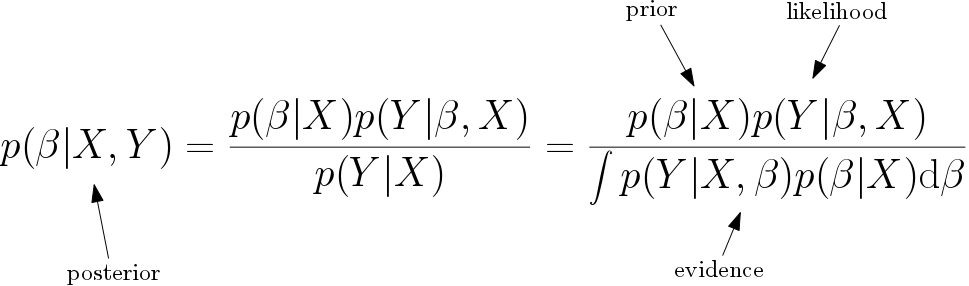
Since the evidence can be written in integral form, we have to pick only two things, the likelihood and the prior distributions. In the linear regression model, we already have a likelihood distribution which is normal with mean \(X\beta\). If we chose our prior to be uniform, i.e. \(p(\beta|X)=1\), and take the maximum of the posterior distribution, then we get the solution \(\hat \beta = (X^TX)^{-1} X^T Y\). More explicitly, we also get a measure of uncertainty for the model, since we know the entire posterior distribution and not just the maximum of the distribution.
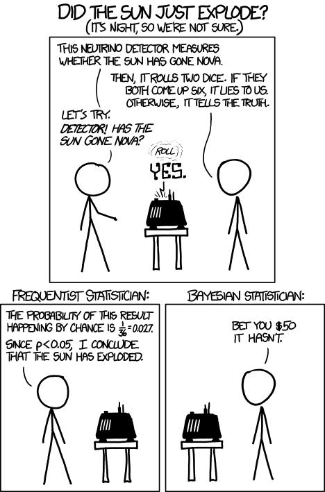
Learning statistics the XKCD way.
How to pick a prior?
Generally there are two reasons for picking a prior, either you have some preconceived ideas about the distribution of \(\beta\), or you want to pick a prior because of some “nice” properties. The first scenario might come up if you have done a similar experiment, or even that you have a posterior from the same experiment done before. For example, if your data comes in batches of 5, you can use the posterior from the previous batch as the prior for the current batch to make the update (which will result in the same posterior as applying the 10 updates all together). As an other example, you might have done an experiment on rats which resulted in a posterior which you can use as a prior for your experiment on humans, since your prior belief is that you expect to get similar results.
The second scenario for priors is a lot more interesting. For example, if we have a lot of predictors, we might want to eliminate some of our predictors, that is, set \(\beta_k=0\), in some systematic way. This will prevent over-fitting and overall will give us a simpler model. Picking a prior which is concentrated at \(0\) achieves just this.
Consider the Laplace distribution as our prior: \(p(\beta | X)=p(\beta) = \prod_{k=1}^p\frac{1}{2\gamma}e^{-|\beta_k|/\gamma}\)
merge(tibble(gamma = c(.2,.5,1,5)), tibble(x = seq(-10,10,0.1)), all = T) %>%
  mutate(y =  exp(-abs(x)/gamma)/(2*gamma),
         gamma = as.factor(gamma)) %>%
  ggplot(aes(x, y, colour = gamma)) +
  geom_line() +
  labs(
    title = 'Density of the Laplace distribution',
    x = 'beta',
    y = 'Density'
  )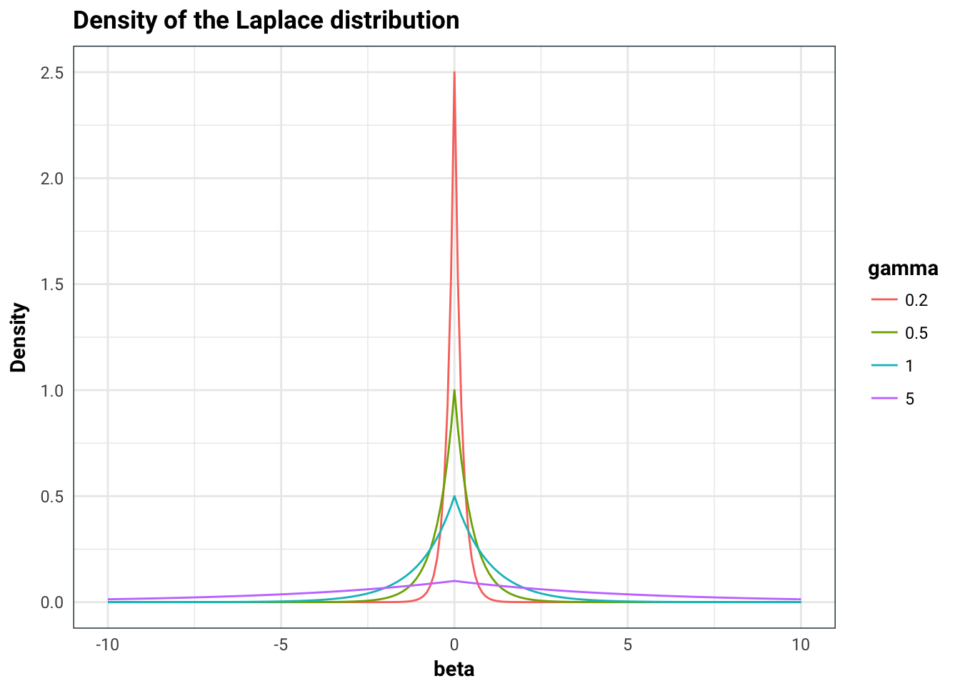
That big old spike concentrated at zero will favour \(\beta_k=0\). It becomes a lot more familiar once we look at the maximum of the posterior
\[ \begin{aligned} \max_\beta p(\beta|X,Y) &= \min_\beta - \log(p(\beta|X,Y)) \\ &= \min_\beta - \log(e^{-\sum_{k=1}^p|\beta_k|/\gamma}e^{-\frac{1}{2}(Y-X\beta)^T(Y-X\beta)}) + \text{const.} \\ &= \min_\beta \frac{1}{\gamma}\sum_{k=1}^p |\beta_k| + \frac{1}{2}(Y-X\beta)^T(Y-X\beta) \end{aligned} \]
which is just the old LASSO resgression.
How to pick a likelihood?
Picking a likelihood equates to picking model. This can go from simple models like linear regression to more complicated models such as deep neural networks. There are some problems in these domains. For example, it is difficult to write down the explicit likelihood function of a deep neural network with many nodes and layers, and even more difficult to consider also pooling layers and other weirdness. There is currently ongoing efforts in trying to understand these complicated models from a Bayesian perspective.
Evidence required
So why would you ever take the maximum of the posterior if you can have the whole posterior? The answer to that is the evidence. That little integral at the bottom is super duper intractable in some cases. Trying to numerically integrate a complicated function in 100 dimensional space is quite a challenging task. Luckily, there are quite a few techniques that make this feasible but that’s a story for an other day.
Turtles all the way down

Let’s go deeper
Of course, we don’t have to stop our Bayesian analysis on just one parameter \(\beta\) that is random. For example, we can impose that \(\beta\), the random parameter we are trying to estimate, itself depends on yet an other variable. This is called hierarchical modeling, as a solid example, take \[ \begin{aligned} \alpha \sim \text{Normal}(0,1)\\ \sigma \sim \text{Exponential}(1)\\ \beta \sim \text{Normal}(\alpha,\sigma) \end{aligned} \] and try to infer the posterior distribution \(p(\alpha, \sigma, \beta | X, Y)\).
I hope that gives a very brief overview of Bayesian statistics. In the upcoming posts, I hope to explore these in more detail. Stay tuned!