Causal impact is a tool for estimating the impact of a one time action. As an example (which we will actually look at the data) consider the BP oil spill in 2010. Let’s say you want to evaluate the impact that this had on BP stocks. Typically with questions like this, we would like to be able to collect multiple samples from a control group and a test group. As this is not possible we would have to try something else.

Intuitively, it would make sense to look at the BP stocks against some benchmark like NASDAQ (I got the data from Yahoo finance):
library(lubridate)
bp <- read_csv('../../data/causal_impact/bp_stocks.csv')
nasdaq <- read_csv('../../data/causal_impact/nasdaq.csv')
stocks <- nasdaq %>%
  select(Date, Open) %>%
  rename(NASDAQ = Open) %>%
  merge(bp %>% select(Date, Open), by = 'Date') %>%
  rename(BP = Open,
         date = Date)
oilSpillDate <- ymd('2010-04-20')
stocks %>%
  gather(stock, price, NASDAQ, BP) %>%
  ggplot(aes(date, price, colour = stock)) +
  geom_vline(xintercept = oilSpillDate, linetype = 'dashed') +
  geom_line() +
  guides(colour = guide_legend(title = NULL)) +
  labs(
    title = 'NASDAQ and BP daily open prices',
    subtitle = 'Oil spil date indicated in dashed line',
    x = '',
    y = 'Price in USD'
  )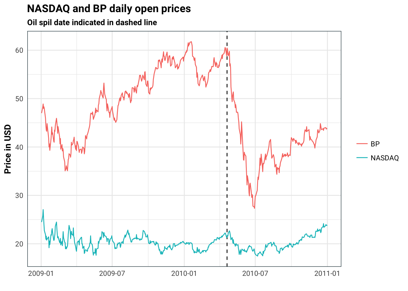
We can see the impact of the oil spill on the stock price of BP. However, how do we estimate the magnitude of this impact? Also, how do we quantify how sure we are?
One idea would be to break the data into two periods, a before and after event. For the before period, we can run a regression against the NASDAQ price, which gives us an idea about the uncertainty:
fittedLM <- lm(BP ~ NASDAQ, data = stocks %>% filter(date < oilSpillDate))
predictLM <- predict(fittedLM, newdata = stocks %>% filter(date == oilSpillDate), interval = 'confidence')
stocks %>%
  mutate(`BP predicted` = ifelse(date < oilSpillDate, NA,  predictLM[1]),
         low = ifelse(date < oilSpillDate, NA,  predictLM[2]),
         high = ifelse(date < oilSpillDate, NA,  predictLM[3])) %>%
  gather(stock, price, BP, NASDAQ, `BP predicted`) %>%
  ggplot(aes(date, price, colour = stock)) +
  geom_vline(xintercept = oilSpillDate, linetype = 'dashed') +
  geom_ribbon(aes(ymin = low, ymax = high), alpha = .2, colour = 'gray') +
  geom_line() +
  guides(colour = guide_legend(title = NULL)) +
  labs(
    title = 'NASDAQ and BP daily open prices',
    subtitle = 'Oil spil date indicated in dashed line',
    x = '',
    y = 'Price in USD'
  )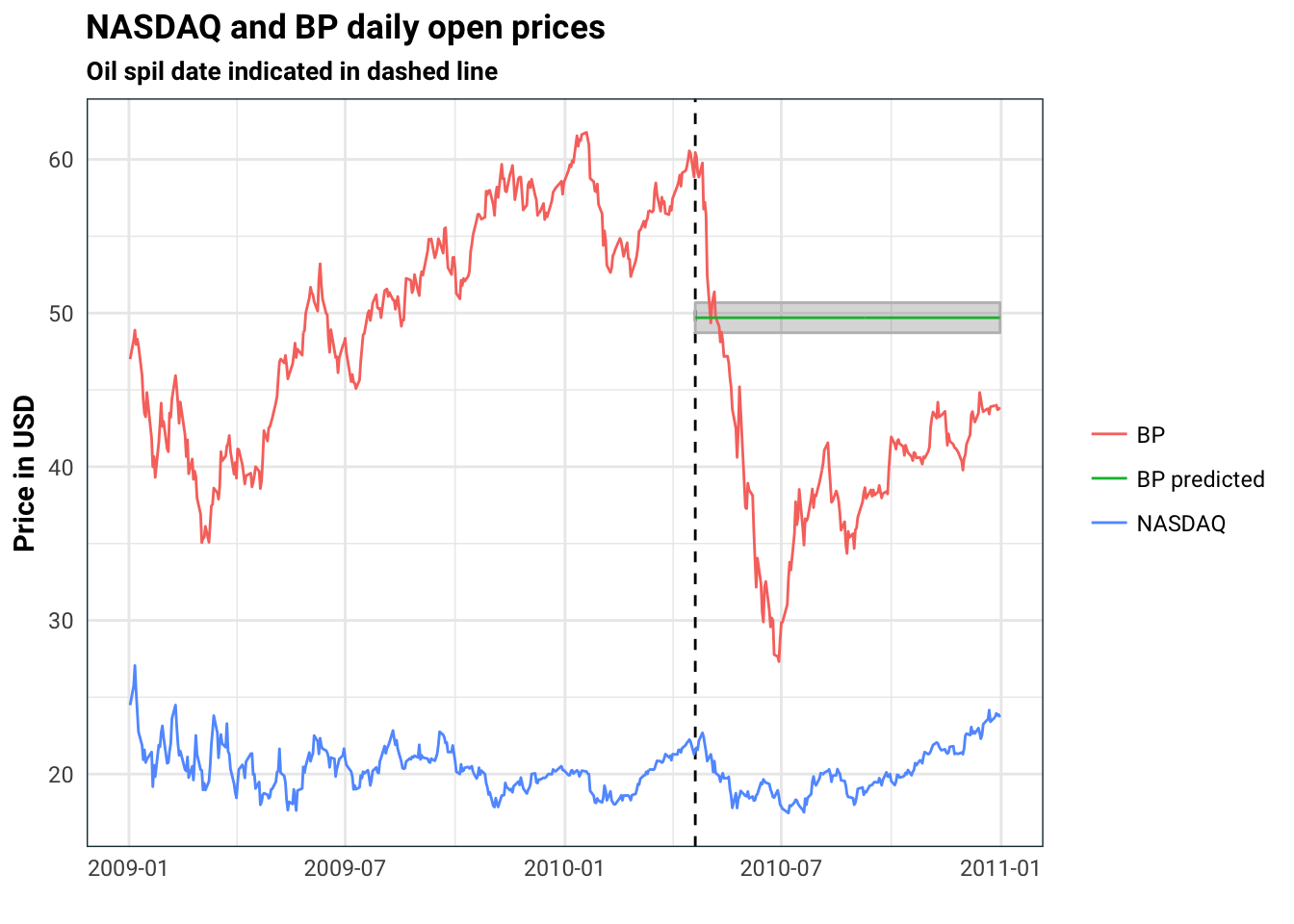
This is rather poor approximation. For one thing, there are all sorts of autocorrelation affects from the times series. Secondly, we have standard error for the estimate, but what we don’t have is a standard error that evolves in time. Obviously, 10 days after the oil spill, I am less certain about the oil spill impact than the day before.

Bayesian structural time series
Instead of a linear model, we can use a time series model. A structural time series model can be described by
\[ \begin{aligned} y_t &= Z_t^T\alpha_t + \epsilon_t \qquad &\epsilon_t \sim N(0, H_t)\\ \alpha_t &= T_t\alpha_{t-1} + R_t\eta_t \qquad &\eta_t \sim N(0, Q_t). \end{aligned} \]
The matrices above are typically partially specified and partially estimated. ARIMA and VARMA models can all be written in the above form. For us, we will use the bsts R package which allows for a one dimensional model for \(y\) of the form:
\[ \begin{aligned} y_t &= \mu_t + \tau_t + \beta^T \mathbf x_t + \epsilon_t\\ \mu_t &= \mu_{t-1} + \delta_{t-1} + \eta_t\\ \delta_t &= \delta_{t-1} + \omega_t\\ \tau_t &= -\sum_{s=1}^{S-1} \tau_{t-s} + \gamma_t. \end{aligned} \]
where \(\epsilon, \eta, \omega, \gamma\) are all independent centred normal random variables, with variances that are the same for all time (but can differ across the four).
There is a lot going on here so lets go through it step by step starting from the bottom equation.
\(\tau\) here is the seasonal component and \(S\) is the number of seasons. Let’s say our data consisted of ice cream sales per season, then \(S=4\) as we would expect each season to have a different baseline for sales (with summer being the highest sales). The sum above means that the total effect of seasonality is zero.
\(\delta_t\) is simply a random walk. This walk denotes the direction of the trend.
\(mu_t\) is the current trend which is compromised of a direction \(\delta_{t-1} + \mu_{t-1}\) plus some noise
\(\mathbf x_t\) is a vector of covariates, that is, other time-series that may help us to better estimate \(y\). In the BP example, we could use the price of Shell Oil company stocks to give us a better estimate for BP stocks. The term \(\beta^T\) can be estimated to form a regression. In fact, in the bsts package, the \(\beta\) is estimated using slab and spike regression. This means that the regression also allows for feature selection meaning we can try to chuck in quite a few terms without having to worry as much about over fitting.
So there are several really cool features of this package. For one thing it’s Bayesian, so we can specify priors. Secondly, it’s super quick. You can see an example usage at the end of this post.
Causal impact
Now that we have a time-series model, a sensible thing to do would be to fit it using the pre-event data. Then we can use that model to predict the post-event path and measure how much that differs from the observed time series. This is exactly what the causal impact package does!
Let us carry on with the BP example we started with. We have two things to work out:
Are there seasonal effects and local trends? If so, how do they behave?
Which other time series do we pick? We need to be careful here. On the one hand, we want \(\mathbf x\) to be highly correlated with \(y\), on the other, we don’t want \(\mathbf x\) to be impacted by the oil spill. So for example, picking Shell stocks might not be best idea because their stocks also take a hit during the spill.
Let’s first just try the vanilla option in causal impact (note there is an issue with irregular time series):
library(CausalImpact)
library(zoo)
stocks.zoo <- stocks[,c(1,3,2)] %>%
  read.zoo()
times <- seq(start(stocks.zoo), end(stocks.zoo), by = 'day')
stocks.zoo <- merge(stocks.zoo, zoo(,times), all = TRUE) %>% na.locf()
impact <- CausalImpact(data = stocks.zoo,
                             pre.period = c(first(stocks$date), oilSpillDate-1),
                             post.period = c(oilSpillDate, last(stocks$date)))
summary(impact)
#> Posterior inference {CausalImpact}
#>
#> Average Cumulative
#> Actual 40 10350
#> Prediction (s.d.) 58 (3.9) 14954 (986.2)
#> 95% CI [51, 66] [12964, 16799]
#>
#> Absolute effect (s.d.) -18 (3.9) -4604 (986.2)
#> 95% CI [-25, -10] [-6449, -2614]
#>
#> Relative effect (s.d.) -31% (6.6%) -31% (6.6%)
#> 95% CI [-43%, -17%] [-43%, -17%]
#>
#> Posterior tail-area probability p: 0.00103
#> Posterior prob. of a causal effect: 99.89733%
#>
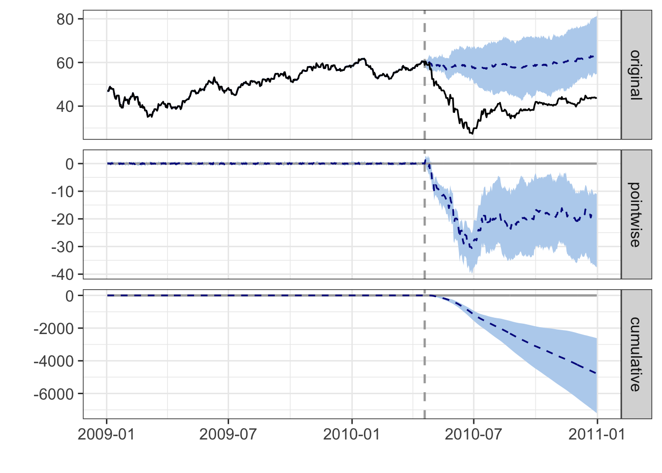
#> For more details, type: summary(impact, "report")plot(impact)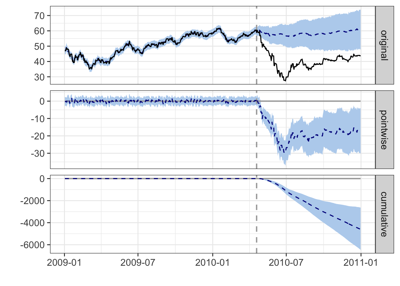
You can also use CasualImpact with your own bsts model:
library(bsts)
stocks.bsts <- stocks.zoo
postPeriod <- which(time(stocks.zoo) == oilSpillDate) : nrow(stocks.zoo)
stocks.bsts[postPeriod, 1] <- NA
ss <- AddLocalLevel(list(), stocks.zoo[,1]) %>%
  AddSeasonal(stocks.zoo[,1], nseasons= 7)

bsts <- bsts(BP ~ NASDAQ, state.specification = ss,
             data = stocks.bsts, niter = 1000)
#> =-=-=-=-= Iteration 0 Sat Feb 3 17:46:37 2018 =-=-=-=-=
#> =-=-=-=-= Iteration 100 Sat Feb 3 17:46:38 2018 =-=-=-=-=
#> =-=-=-=-= Iteration 200 Sat Feb 3 17:46:39 2018 =-=-=-=-=
#> =-=-=-=-= Iteration 300 Sat Feb 3 17:46:41 2018 =-=-=-=-=
#> =-=-=-=-= Iteration 400 Sat Feb 3 17:46:42 2018 =-=-=-=-=
#> =-=-=-=-= Iteration 500 Sat Feb 3 17:46:44 2018 =-=-=-=-=
#> =-=-=-=-= Iteration 600 Sat Feb 3 17:46:46 2018 =-=-=-=-=
#> =-=-=-=-= Iteration 700 Sat Feb 3 17:46:47 2018 =-=-=-=-=
#> =-=-=-=-= Iteration 800 Sat Feb 3 17:46:49 2018 =-=-=-=-=
#> =-=-=-=-= Iteration 900 Sat Feb 3 17:46:50 2018 =-=-=-=-=impact.bsts <- CausalImpact(bsts.model = bsts,
post.period.response = stocks.zoo[postPeriod,1] %>% as.numeric())
plot(impact.bsts)