In this post we take a look at the summer Olympics and try to see which countries performed substantially differently than was expected of them. We will look at the Olympics from 1964 through to 2008. For each year, we will run a predictive model, trying to predict the number of medals a country wins, using selected datasets that are available before each of the Olympics. We will see that this model performs well out of sample and this model will be what we expect. We can see which countries performed better than expected, for example, by looking at which countries perform better than the model predictions. If you are into your Latin, this is called ex-ante (before the event) which is in contrast with ex-post (after the facts). Let’s stop getting hung up on the exes, it’s time to move on.

OK so ideally we would like to predict the number of medals that a country is going to win. The first problem with this is that the number of medals handed out differs from year to year.
medals <- read_csv('../../data/olympics/medals.csv')
medals %>%
  group_by(Edition, Gender) %>%
  summarise(number_of_medals = n()) %>%
  ggplot(aes(Edition, number_of_medals, colour = Gender)) +
  geom_line() +
  geom_point() +
  labs(
    title = 'Number of Olympic medals handed out',
    x = 'Year',
    y = 'Number of medals handed out'
  )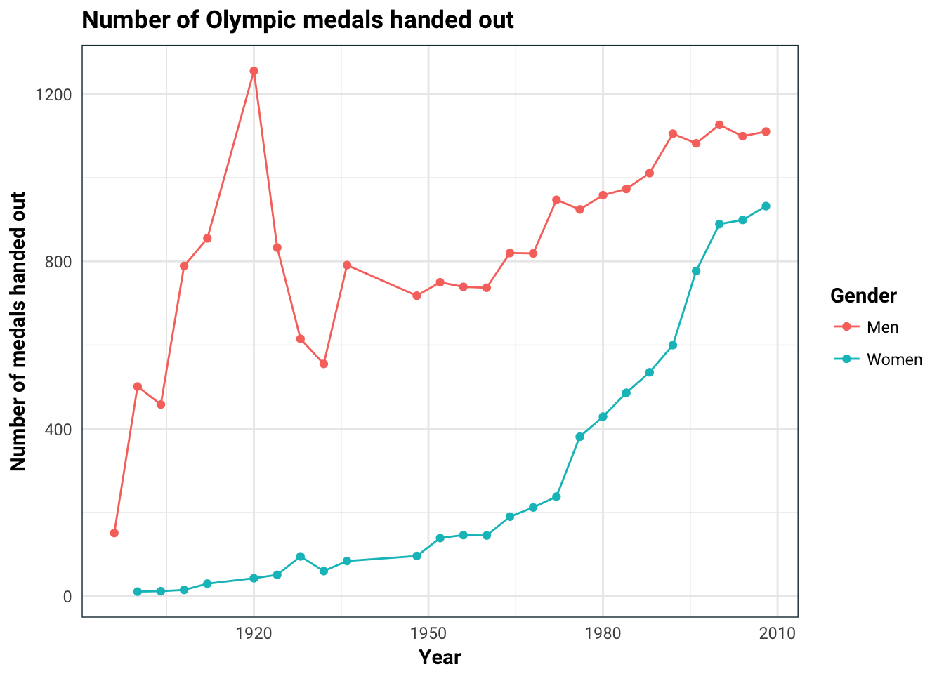
This is going to be a problem since 10 medals won in 2008 is not as impressive as 10 medals won in 1896 since there are way more medals being handed out in 2008 (for both men and women).
An other thing we have to be careful of is that the number of countries competing in the Olympics might not be the same. The graph below indicates this.
medals %>%
  group_by(Gender, Edition) %>%
  summarise(number_of_countries = length(unique(NOC))) %>%
  ggplot(aes(Edition, number_of_countries, colour = Gender)) +
  geom_line() +
  geom_point() +
  labs(
    title = 'Number of countries receiving medals',
    x = 'Year',
    y = 'Number of unique countries receiving medals'
  )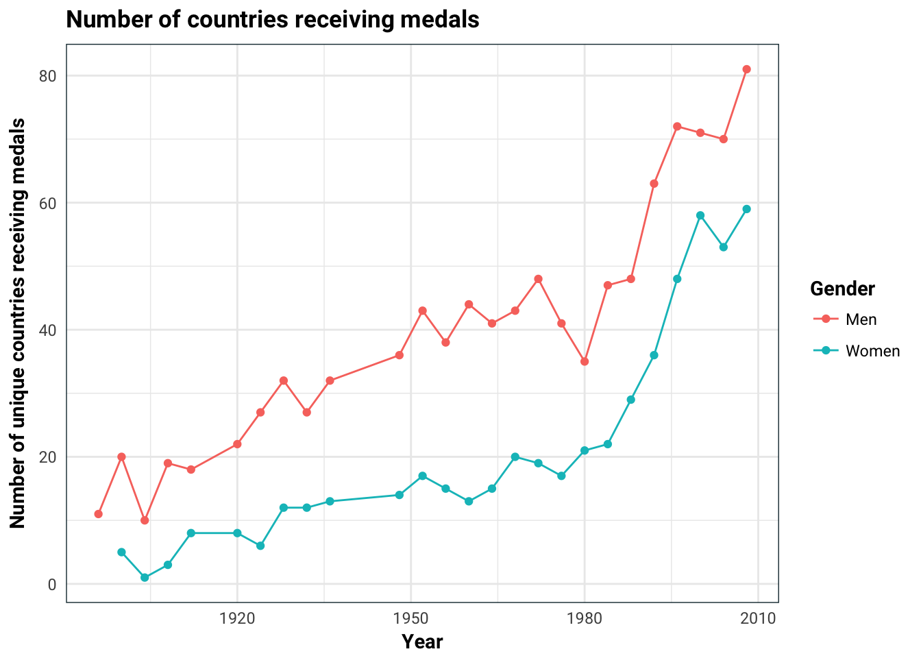
Unfortunately, I couldn’t get hold of any dataset that lists the countries that participated in the Olympics by year. Instead we will make a rather blunt assumption that the countries that participated are the ones that won at least one medal. For each country and year, we will calculate the number of medals it won. Naively, we can guess how many medals each country should win, for example, if there are 4 competing countries and 70 medals handed out one year, I would naively guess that each of them to win 70/4 many medals. Then our response will be calculated as
\[ Y = \frac{\text{Number of medals won} - \text{Naive guess}}{\text{Naive guess}}. \]
medals.response <- medals %>%
  group_by(Edition) %>%
  mutate(total_medals = n(),
         naive_no_medals = total_medals / length(unique(NOC))) %>%
  group_by(Edition, NOC) %>%
  summarise(number_of_medals = n(),
            total_medals = first(total_medals),
            naive_no_medals = first(naive_no_medals),
            response = (number_of_medals -  naive_no_medals) / naive_no_medals)
This isn’t quite ex-ante, since we are using the number of countries that won at least one medal in that year and this information is only available after the Olympics is completed. Ideally, it would be ex-ante if we knew which countries are competing in the Olympics, which is available earlier.
Modelling
Now that we have a response variable, it’s time to build a model. Let’s think for a second what would help to predict a counties performance in the Olympics.

At this point, we just want to get some features that may contribute to the predictive model. We can leave the feature selection to the models. Remember, there are no stupid ideas, just stupid people.
- Previous Olympics performance: pretty self explanatory why it would be important. When we don’t have this data, we will assume the naive guess above (i.e. the response is zero).
- Population: the more people a country has, the more chance it has of having competitive athletes
- GDP: many of the events require special equipment that only rich countries can afford. Since we will use population, it makes sense to use GDP per capita instead of GDP
- Climate: A lot of the events are geared towards outdoors so climate could be a factor. This can be somewhat ambiguous for large countries (I’m looking at you USA). This is also something that is somewhat stationary and thus the effects may be captures by the previous Olympics performance so we will leave it out.
- Percentage of people in urban areas: It seems to me that the Olympic games are an urban thing and thus performance is benefited from having more urban dwellers.
We will use the statistics about the countries that were compiled for the year prior to the year in which the Olympic games were held.
read_wb_table <- function(file_name) {
  file_path <- paste0('../../data/olympics/', file_name, '.csv')
  read_csv(file_path) %>%
    select(-X63) %>%
    gather('Edition', value, -`Country Name`, -`Country Code`, -`Indicator Name`, -`Indicator Code`) %>%
    select(Edition, `Country Name`, value) %>%
    mutate(Edition = as.integer(Edition) + 1,
           value = as.numeric(value)) %>%
    set_names(c('Edition', 'country_name', file_name))
}
files <- c('population', 'gdp_per_capita', 'urban_population')
olympics <- lapply(files, read_wb_table)
olympics <- Reduce(function(x,y) full_join(x,y, by = c('Edition', 'country_name')), olympics) %>%
  as.tibble
dictionary <- read_csv('../../data/olympics/dictionary.csv') %>%
  rename(country_name = Country,
         NOC = Code)
olympics <- left_join(olympics, dictionary, by = 'country_name')
olympics <- inner_join(medals.response, olympics, by = c('Edition', 'NOC'))
The data on the countries from the world bank is from 1960 onwards and this gives us 575 data points.
olympics.data <- olympics %>%
  group_by(NOC) %>%
  mutate(prev_performance = lag(response),
         prev_performance = replace(prev_performance, is.na(prev_performance), 0)) %>%
  ungroup() %>%
  select(response, population, urban_population, gdp_per_capita, prev_performance)
olympics.data %>%
  cor(use = 'pairwise.complete.obs') %>%
  corrplot::corrplot.mixed()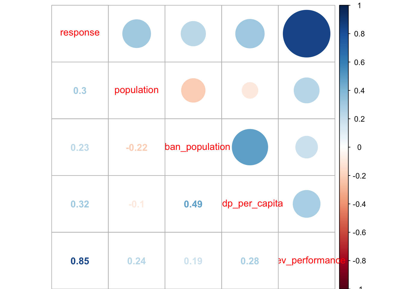
library(mlr)
task <- makeRegrTask(data = olympics.data, target = 'response')
task.imp <- generateFilterValuesData(task, 'randomForestSRC.rfsrc')
plotFilterValues(task.imp) +
  labs(
    title = 'Feature importance according to random forest',
    x = 'Feautre',
    y = 'Importance value'
  )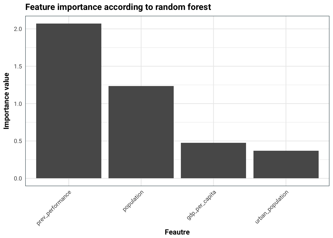
We can immediately see that the previous performance is most likely the best feature. The urbanisation of the country is also quite heavily correlated with the GDP per capita, which is expected.
Next, we could try to fit many models and use the one that gives best out of sample. This will also also involve imputing the missing data since many models cannot handle missing data. However, for this post I am going to be a bit lazy and only use a random forest model.
We will use bootstrapping to get an estimate of how good this model is. We will compare the performance of the model against the simple model where the next response is predicted to be the previous response.
rf <- makeLearner('regr.randomForestSRC')

mse_on_boot <- function(ind) {
  fit <- train(rf, task, subset = ind)
  oob <- (1:nrow(olympics.data))[-ind]
  preds <- predict(fit, task, subset = oob)
  mse_basic <- with(olympics.data[oob,], mean((response - prev_performance)^2))
  1 - performance(preds, measures = list(mse)) / mse_basic
}
boots <- tibble(iter = 1:25) %>%
  mutate(rsq = map_dbl(iter, ~sample(1:nrow(olympics.data), nrow(olympics.data), replace = T) %>% mse_on_boot()))
boots %>%
  ggplot(aes(rsq)) +
  geom_histogram(binwidth = .1) +
  labs(
    title = 'Bootstrapped performance of the model',
    x = 'R squared against previous performance',
    y = 'Count'
  )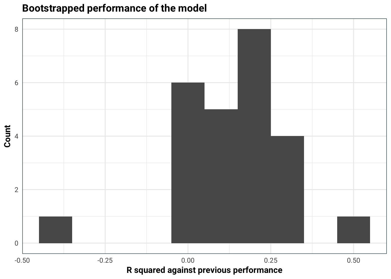
Our model explains about 15-20% of the variance left over from simply predicting the next Olympic games result is the same as the current one. This is pretty good!
The 2008 surprises
Now let’s take a look at the 2008 games and see which countries performed different to expectations. We will train the model on the data set excluding 2008 and then use the model to predict 2008. Then we will single out the countries that did substantially differently than expected.
train_ind <- which(olympics$Edition != 2008)
predict_ind <- which(olympics$Edition == 2008)
rf.fit <- train(rf, task, subset = train_ind)
preds <- predict(rf.fit, task, subset = predict_ind)
surprise <- preds$data %>%
  mutate(diff = abs(truth - response)) %>%
  arrange(-diff) %>%
  slice(1:10) %>%
  select(id, pred = response)
left_join(surprise, olympics %>% ungroup() %>%  mutate(id = 1:n()), by = 'id') %>%
  mutate(pred = pred * naive_no_medals + naive_no_medals) %>%
  mutate(diff = pred - number_of_medals) %>%
  select(Country = country_name, `Actual number` = number_of_medals, `Predicted` = pred, diff) %>%
  gather(type, value, -Country, -diff) %>%
  ggplot(aes(reorder(Country, -diff), value, fill = type)) +
  geom_col(position = 'dodge', colour = 'black') +
  labs(
    title = 'Biggest surprises of the 2008 Olympics',
    x = 'Country',
    y = 'Number of medals'
  ) +
  guides(fill = guide_legend(title = NULL)) +
  theme(
    axis.text.x = element_text(angle = -45, hjust = 0, vjust = 1)
  )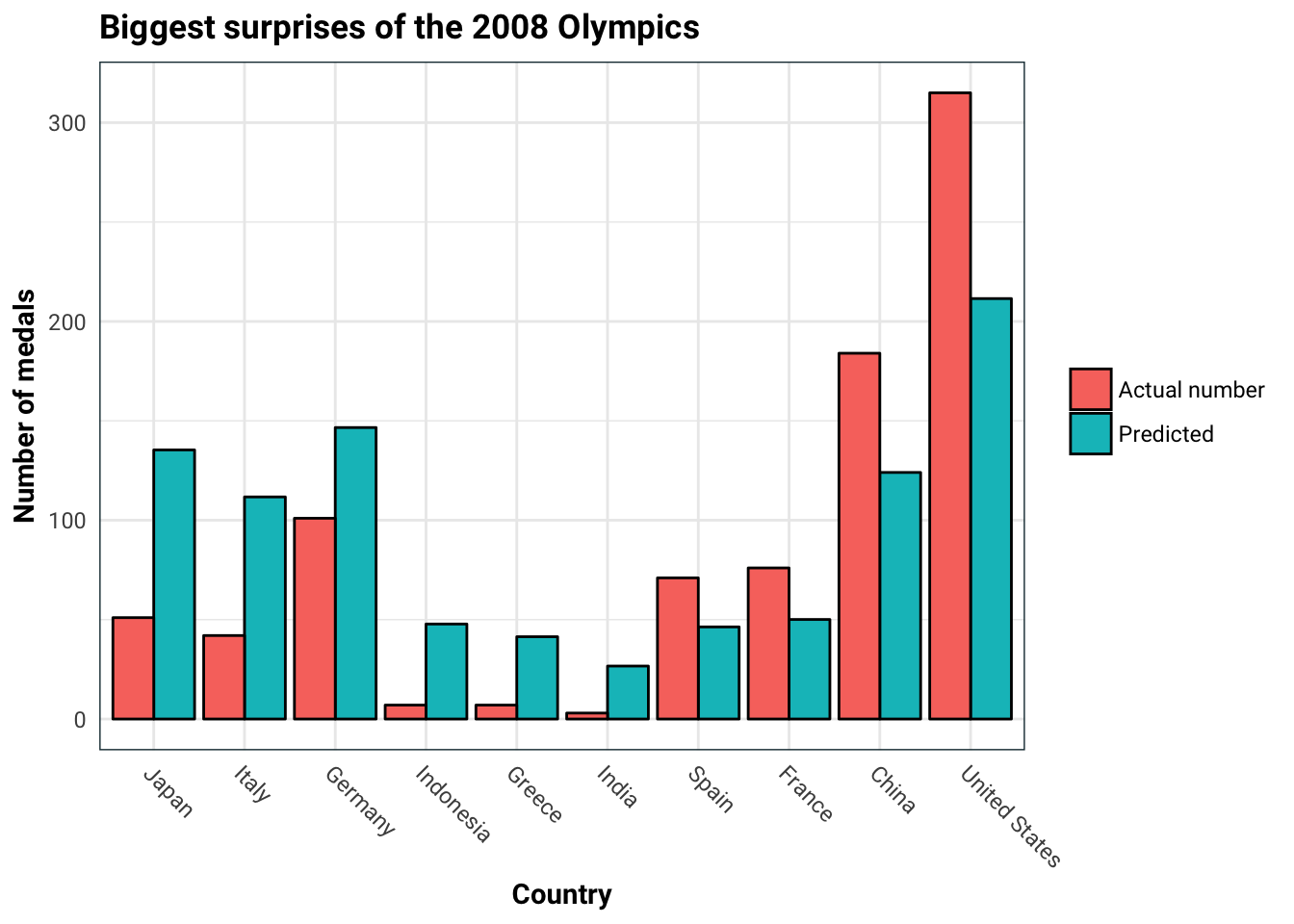
It seems that Japan and Italy performed way below expectations, whereas USA and China performed above expectations.
The surprising years
We can also see which were the years that we should have watched the Olympics. For this, we will look at the games between 1980-2008. We will do ex-ante predictions, meaning, we only train on the years before.
years <- unique(olympics$Edition)
analyse_years <- years[years >= 1980]
rolling <- lapply(analyse_years, function(year){
  train_ind <- which(olympics$Edition < year)
  predict_ind <- which(olympics$Edition == year)
  rf.fit <- train(rf, task, subset = train_ind)
  preds <- predict(rf.fit, task, subset = predict_ind)
  preds <- preds$data %>%
    select(id, pred = response)
  left_join(preds, olympics %>% ungroup() %>%  mutate(id = 1:n()), by = 'id') %>%
    mutate(pred = pred * naive_no_medals + naive_no_medals) %>%
    mutate(abs_diff = abs(pred - number_of_medals)) %>%
    group_by(Edition) %>%
    summarise(mae = mean(abs_diff))
}) %>%
  do.call(rbind, .)
rolling %>%
  ggplot(aes(Edition, mae)) +
  geom_line(colour = .colr[2]) +
  geom_point(colour = .colr[3]) +
  labs(
    title = 'The absolute difference between expected and realised number of medals',
    x = 'Year',
    y = 'Mean absolute difference between predicted and actual'
  )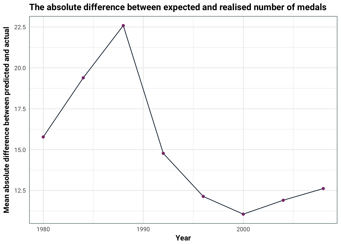
It looks like 1988 was the year to watch!

Sources
This post was inspired by the More or Less episode. Feel free to check out this awesome paper for further (and better) examples of the type of ex-ante analysis performed here.