In this post we are going to look at some football statistics. In particular, we will examine English football, the Premier League, using Bayesian statistics with Stan. If you have no idea what Bayesian statistics is, you can read my introductory post on it. Otherwise this post shouldn’t be a difficult read.
All right, let’s get to it. First, we need some data. I will use all the matches from the Premier League seasons 16/17 and 17/18 (which is still ongoing at the time of the writing). You can find the data yourself in the sources listed at the bottom.
football.2017 <- read_csv('../../data/football/premier2017.csv') %>%
  mutate(season = '16/17')
football.2018 <- read_csv('../../data/football/premier2018.csv') %>%
  select(-starts_with('X')) %>%
  mutate(season = '17/18')
football <- rbind(football.2017, football.2018) %>%
  as.tibble()
football %>%
  select(season, HomeTeam, AwayTeam, FTHG, FTAG) %>%
  DT::datatable(caption = 'Combined data for 16/17 and 17/18 season games',
                options = list(pageLength = 5))
Above, we just joined the two seasons of data (for some reason the 17/18 season came with two extra columns). Using the columns FTHG = full time home goals and FTAG = full time away goals, we can see what the current 17/18 season standings look like:
football.standings <- football %>%
  mutate(home_points = ifelse(FTHG > FTAG, 3, ifelse(FTHG == FTAG, 1, 0)),
         away_points = ifelse(home_points == 3, 0, ifelse(home_points == 1, 1, 3))) %>%
  gather(side, team, HomeTeam, AwayTeam) %>%
  mutate(points = ifelse(side == 'HomeTeam', home_points, away_points)) %>%
  group_by(season, team) %>%
  summarise(points= sum(points),
            played = n()) %>%
  ungroup()

football.standings %>%
  filter(season == '17/18') %>%
  arrange(-points) %>%
  mutate(position = 1:n()) %>%
  select(position, team, played, points) %>%
  DT::datatable(caption = 'Standings for the 17/18 season',
                options = list(pageLength = 8))
You can probably guess who is going to be champion, so let’s focus on something else. Let’s take a look at how to model the full time results of each match. For this we are going to do a rather simple model. Each team will have a parameter \(\lambda_j\) which we call prowess. Let say Manchester Utd is playing Manchester City, then we will assume that both Utd and City score goals independently according to Poisson distributions Po\((\lambda_{{Utd}})\) and Po\((\lambda_{{City}})\) respectively. Then the score difference is given by a Skellam distribution which is just the difference between independent Poisson random variables. So our response will be the goal difference. Moreover, we will make this signed so that it’s the home team goals minus the away team goals.
OK OK, I can hear you groaning in agony about this model. There are teams that win games by scoring goals and teams that win by defending, so a team with a really good defence might get a high prowess simply because the model makes no distinction between the result 1-0 and the result 4-3. So under our Poissonian explanation, it might appear that they are assumed to score more goals which is not true. Though I think this effect will somewhat be cancelled out when we look at the difference of the Poisson random variables.

y <- football$FTHG - football$FTAG
N <- length(y)
teams <- unique(football$HomeTeam)
team1 <- match(football$HomeTeam, teams)
team2 <- match(football$AwayTeam, teams)
Nteams <- length(teams)
library(rstan)
options(mc.cores = parallel::detectCores())
Now we have Stan ready to go, let’s discuss what we are going to do. First, in formulas:
\[ \begin{aligned} \sigma_i &\sim \text{Inverse-}\Gamma(1,1)\\ \lambda_i &\sim \text{Log-Normal}(\mu_{\text{prior}_i}, \sigma^2_i)\\ y &\sim \text{Skellam}(\lambda_{\text{Home team}},\lambda_{\text{Away team}}) \end{aligned} \]
Let’s go through this. We will try infer the the prowess of each team \(\lambda\). As stated before, we assume that the outcome of the matches, which are the score differences between the home and away team is given by a Skellam distribution with the appropriate parameters. Next we need to pick prior distributions for \(\lambda\). For this, we assume that \(\lambda\) is Log-Normal with a median which we will prescribe before hand by manually setting some of the top teams to have higher \(\mu\). For the \(\sigma\) parameter, we use a hierarchical model and give that a prior of inverse gamma distribution.
First, let’s specify which teams we expect to be stronger. Here I will keep it simple. I will separate the teams into three by my own intuition: top, mid, and other The top teams get a median of 1.5 (the median is given by \(e^\mu\)), middle get median of 1.3 and the others will get a median of 1. If your favourite team isn’t listed how you would have done it, don’t worry too much, this prior selection doesn’t affect the analysis that much.
prior_mu <- rep(0, length(teams))
top_teams <- c('Arsenal', 'Chelsea', 'Man United', 'Liverpool', 'Man City', 'Tottenham')
med_teams <- c('Everton', 'Southampton', 'Leicester')
prior_mu[match(top_teams, teams)] <- log(1.5)
prior_mu[match(med_teams, teams)] <- log(1.3)
With all of that done. We can now use Stan to compile and fit the model.
functions {
  real skellam_log(int k, real lambda1, real lambda2) {
    real r = k;
    return -(lambda1 + lambda2) + (r/2) * log(lambda1/lambda2) +
      log(modified_bessel_first_kind(k, 2 * sqrt(lambda1 * lambda2)));
  }
}
data {
  int<lower=0> N;
  int<lower=0> Nteams;
  int<lower=0> team1[N];
  int<lower=0> team2[N];
  real<lower=0> prior_mu[Nteams];
  int y[N];
}
parameters {
  real<lower=0> lambda[Nteams];
  real sigma;
}
model {
  sigma ~ inv_gamma(1,1);
  lambda ~ lognormal(prior_mu, sigma^2);
  for(i in 1:N)
    y[i] ~ skellam(lambda[team1[i]], lambda[team2[i]]);
}
stan.fit <- sampling(stan.model)library(stringr)
posterior_draws <- stan.fit %>%
as.data.frame() %>%
as.tibble() %>%
select(starts_with('lambda')) %>%
gather(param, draw, everything()) %>%
mutate(param = str_replace_all(param, '[^0-9]', '') %>% as.integer())
posterior_draws %>%
group_by(param) %>%
summarise(median = median(draw), up = quantile(draw, .95), down = quantile(draw, .05)) %>%
mutate(team = map_chr(param, ~teams[.])) %>%
ggplot(aes(reorder(team, median), median)) +
geom_errorbar(aes(ymin = down, ymax = up), colour = .colr[3]) +
geom_point(colour = .colr[2]) +
coord_flip() +
labs(
title = 'Seasons 16/17 and 17/18 Premier League team prowesses',
subtitle = 'Median and the 95% credible interval',
y = 'Prowess',
x = ''
)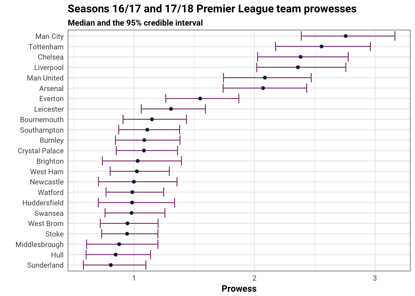
No surprises for guessing the top teams in prowess: Man City, Chelsea, Liverpool, Man Utd, Arsenal, Tottenham and Liverpool. On the other end of the spectrum, Sunderland, Middlesbrough and Hull got relegated in the 2016/2017 season, so it’s no surprise seeing them at the bottom.
Next we can take a look at home advantage.

In the Bayesian world we can do this in a rather neat way. For each team we will have three parameters, \(\gamma \in [0,1]\), \(\lambda^h, \lambda^a \geq 0\). In the previous model, the prowess parameter \(\lambda\) did not depend on if the team was playing at home or away. Now we split this into two, \(\lambda^h\) and \(\lambda^a\). Additionally, each team has a parameter \(\gamma\) which determines how much (if any) home prowess differs from away prowess.
\[ \begin{aligned} \sigma_i, \tilde \sigma_i &\sim \text{Inverse-}\Gamma(1,1)\\ \lambda^h_i &\sim \text{Log-Normal}(\mu_{\scriptsize\text{prior}_i}, \sigma^2_i)\\ \lambda^a_i &\sim \text{Log-Normal}(0.9\cdot\mu_{\scriptsize\text{prior}_i}, \tilde\sigma^2_i)\\ \gamma &\sim U[0,1]\\ W &\sim \text{Bernoilli}(\gamma_{\scriptsize\text{Away team}})\\ y &\sim W\cdot \text{Skellam}(\lambda^h_{\scriptsize \text{Home team}},\lambda^a_{\scriptsize\text{Away team}}) \\ &\quad+ (1-W) \cdot \text{Skellam}(\lambda^h_{\scriptsize\text{Home team}},\lambda^h_{\scriptsize\text{Away team}}) \end{aligned} \]
We can see from the above that if \(\gamma = 0\) then the team has the same prowess at home as away. The parameter \(\gamma\) in general controls how significant the difference between the home and away prowess of a team is. Simply put, it is the probability that the team will perform significantly different at home than away.
functions {
  real skellam_lpmf(int k, real lambda1, real lambda2) {
    real r = k;
    return -(lambda1 + lambda2) + (r/2) * log(lambda1/lambda2) +
      log(modified_bessel_first_kind(k, 2 * sqrt(lambda1 * lambda2)));
  }
}
data {
  int<lower=0> N;
  int<lower=0> Nteams;
  int<lower=0> team1[N];
  int<lower=0> team2[N];
  vector[Nteams] prior_mu;
  int y[N];
}
parameters {
  real<lower=0> lambda_home[Nteams];
  real<lower=0> lambda_away[Nteams];
  real<lower=0,upper=1> gamma[Nteams];
  real sigma_home;
  real sigma_away;
}
model {
  sigma_home ~ inv_gamma(1,1);
  sigma_away ~ inv_gamma(1,1);
  lambda_home ~ lognormal(prior_mu, sigma_home^2);
  lambda_away ~ lognormal(0.9 * prior_mu, sigma_away^2);
  for(i in 1:N){
    target += log_mix(gamma[team2[i]],
            skellam_lpmf(y[i] | lambda_home[team1[i]], lambda_away[team2[i]]),
            skellam_lpmf(y[i] | lambda_home[team1[i]], lambda_home[team2[i]]));
  }
}
stan_home_away.fit <- sampling(stan_home_away.model)
stan_home_away.fit %>%
  as.data.frame() %>%
  as.tibble() %>%
  select(starts_with('gamma')) %>%
  gather(param, draw, everything()) %>%
  mutate(param = str_replace_all(param, '[^0-9]', '') %>% as.integer()) %>%
  group_by(param) %>%
  summarise(median = median(draw), up = quantile(draw, .95), down = quantile(draw, .05)) %>%
  mutate(team = map_chr(param, ~teams[.])) %>%
  ggplot(aes(reorder(team, median), median)) +
  geom_errorbar(aes(ymin = down, ymax = up), colour = .colr[1]) +
  geom_point(colour = .colr[5]) +
  coord_flip() +
  labs(
    title = 'Seasons 16/17 and 17/18 probability of different performances',
    subtitle = 'Median and the 95% credible interval',
    y = 'Probability of the team performing differently at home and away',
    x = ''
  )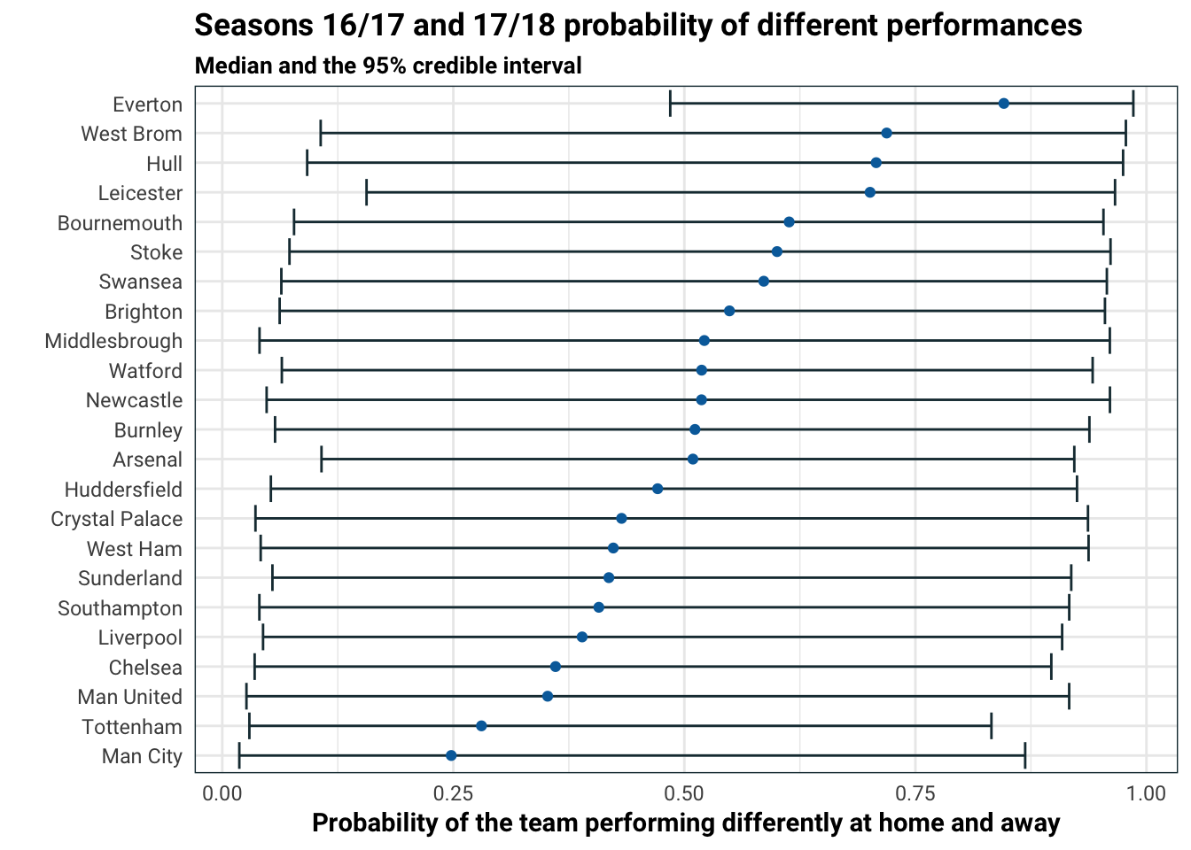
We can see that Everton is by and large the team with the most difference in their home and away performances. Then West Brom, Hull and Leicester have a smaller but still quite large difference. On the other side of it, Man City, Man Utd and Tottenham play pretty consistently between home and away games.
stan_home_away.fit %>%
  as.data.frame() %>%
  as.tibble() %>%
  select(starts_with('lambda')) %>%
  mutate(id = 1:n()) %>%
  gather(param, draw, starts_with('lambda')) %>%
  mutate(param_num = str_replace_all(param, '[^0-9]', '') %>% as.integer()) %>%
  mutate(param_name = str_replace_all(param, '[\\[\\]0-9]', '') %>% as.factor()) %>%
  mutate(team = map_chr(param_num, ~teams[.])) %>%
  select(-param, -param_num) %>%
  spread(param_name, draw) %>%
  mutate(diff = lambda_home - lambda_away) %>%
  group_by(team) %>%
  summarise(median = median(diff), up = quantile(diff, .95), down = quantile(diff, .05)) %>%
  ggplot(aes(reorder(team, median), median)) +
  geom_errorbar(aes(ymin = down, ymax = up), colour = .colr[6]) +
  geom_point(colour = .colr[1]) +
  coord_flip() +
  labs(
    title = 'Seasons 16/17 and 17/18 difference between home and away prowess',
    subtitle = 'Median and the 95% credible interval',
    y = 'Home prowess - Away prowess',
    x = ''
  )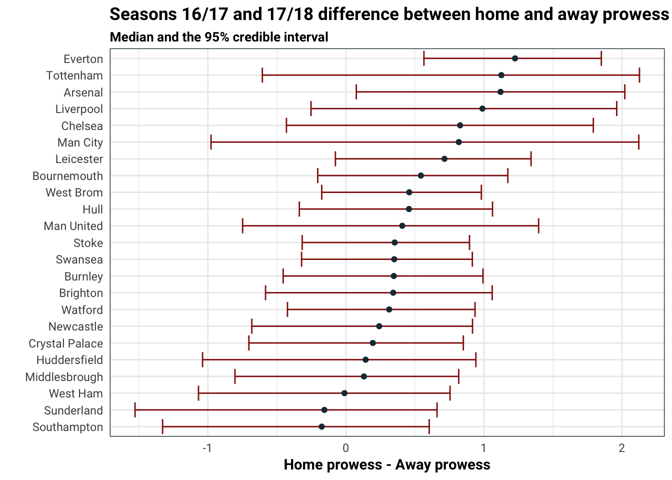
The only two teams with significant change between the home prowess and away prowess are Arsenal and Everton. This is because the 95% credible interval excludes the point 0. Together with the \(\gamma\) plot, we can see that Everton’s Achilles heel is dropping points on away matches. Combined with their general prowess, we can see that Everton perform like the top teams in the league at home, but perform poorly on away matches, which we can actally see in the news. Arsenal also suffers from a similar issue, but less so than Everton.
Note that Sunderland and Southampton both have negative median for the difference, which means that they tend to play better away than at home. Though we can’t be very sure of this since this could be due to a handful of heavy home defeats or away wins.
Well that’s it for today folks. I know we have barely scratched the surface, but I hope that this post has given you some cool stuff you can do with Bayesian analysis.