Spike and slab is a Bayesian model for simultaneously picking features and doing linear regression. Spike and slab is a shrinkage method, much like ridge and lasso regression, in the sense that it shrinks the “weak” beta values from the regression towards zero. Don’t worry if you have never heard of any of those terms, we will explore all of these using Stan. If you don’t know anything about Bayesian statistics, you can read my introductory post before reading this one.
Our tale begins in a land most familiar to us, with just plain old linear regression: \[ y = X\beta + \epsilon \] where \(\epsilon\) is a vector of iid normal distributions \(N(0, \sigma^2)\). Except that we are going to write this in a different, but equivalent way: \[ y \sim N(X \beta, \sigma^2). \] Why you might ask. Well, firstly, this makes the model much easier to extend. For example, we can replace the normal distribution with a t-distribution if we suspect that the data has heavier tails. Secondly, it makes it explicit that \(y\) is modelled as random.
Now since we are full Bayesian, we need a prior for \(\beta\). There are several choices we can make.
data {
  int<lower=0> n;
  int<lower=0> p;
  real y[n];
  matrix[n, p] X;
}
parameters {
  vector[p] beta_flat;
  vector[p] beta_normal;
  vector[p] beta_laplace;
  real<lower=0> sigma_flat;
  real<lower=0> sigma_normal;
  real<lower=0> sigma_laplace;
}
model {
  beta_normal ~ normal(0,1);
  beta_laplace ~ double_exponential(0,1);
  y ~ normal(X * beta_flat, sigma_flat);
  y ~ normal(X * beta_normal, sigma_normal);
  y ~ normal(X * beta_laplace, sigma_laplace);
}
library(rstan)
library(stringr)
options(mc.cores = parallel::detectCores())
simple_reg.data <- list(n = 100, p = 1)
simple_reg.data$X <- with(simple_reg.data, matrix(rnorm(n = n*p), n, p))
simple_reg.data$beta <- 1.7
simple_reg.data$y <- with(simple_reg.data, X %*% beta + rnorm(n = n, sd = 10))[,1]
simple_reg.fit <- sampling(simple_reg, data = simple_reg.data, show_messages=F)
posterior <- simple_reg.fit %>%
extract() %>%
as.data.frame() %>%
as.tibble() %>%
mutate(prior_flat = runif(4000, -5, 5),
prior_normal = rnorm(4000, 0, 1),
prior_laplace = rmutil::rlaplace(4000, 0, 1)) %>%
select(-`lp__`, -starts_with('sigma')) %>%
gather(variable, sample, everything()) %>%
mutate(type = str_replace(variable, '[^_]*', '') %>% substring(2)) %>%
mutate(variable = str_replace(variable, '_[a-z]+', ''),
variable = replace(variable, variable == 'beta', 'posterior'))
ggplot(posterior, aes(sample, variable, fill = variable)) +
ggridges::geom_density_ridges() +
geom_vline(xintercept = simple_reg.data$beta, linetype = 'dashed', colour = 'red') +
facet_wrap(~type) +
coord_cartesian(xlim = c(-4, 4)) +
guides(fill = F) +
labs(
title = 'Density of the prior and posterior',
x = '',
y = ''
)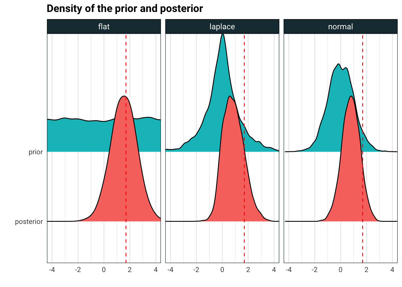
So what is going on here? A flat prior will give a posterior which is normal, with mean at the solution of the ordinary least squares. Laplace and normal priors shrink the mode of the posterior towards zero. In fact, the mode of the posterior is the solution to lasso regression when the prior is Laplace and the ridge regression when the prior is normal. The degree of shrinkage is controlled by the variance of the prior, the lower the variance, the more we shrink to zero.
OK, so that’s pretty neat. Now consider the problem where we have a lot of features that we want to eliminate. We think that only a subset of these are relevant, and the features also have a non-trivial interaction. Think about trying to predict someone’s life expectancy from their genes.

Genes can predict some things with surprising accuracy
There are too many features to just iterate through the subsets and see which one fits the best. So now you might say, just use a lasso regression and drop the the smaller terms. Or even to use the LARS path and select the say the first k that are added to the model. This is unsatisfactory for three reasons: (1) any feature with small, but significant impact is likely going to get dropped and (2) requires cross validation k which may or may not be great and (3) we have absolutely no idea about the uncertainty. Of course, these are not fatal flaws, can be fixed, but instead here we look at a Bayesian approach to the problem.
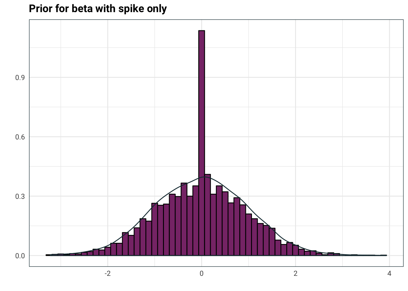
The idea is simple, we set the prior of \(\beta\) to have mass at zero, meaning \(\mathbb P(\beta = 0)>0\) so that the prior distribution of \(\beta\) is a combination of a discrete and continuous density. Formally,
\[ \begin{aligned} \beta_i &= \xi_i \cdot Z_i\\ \xi_i &\sim \text{Bernoulli}_{\{0,1\}}(p_i)\\ Z_i &\sim N(0, \Sigma). \end{aligned} \]
This is the spike in spike and slab (because the distribution spikes at zero). So what’s the slab? Well we haven’t specified \(\Sigma\) yet and this is where the slab comes from.

Let’s crunch in the slab
If we were to throw in a fixed \(\Sigma\), this is what the prior would look like:
tibble(
  xi = rbernoulli(n = 4000, p = .9),
  Z = rnorm(n = 4000),
  beta = Z * xi
) %>%
  ggplot(aes(beta)) +
  geom_histogram(aes(y=..density..), colour = 'black', fill = .colr[3], binwidth = .125) +
  geom_density(aes(replace(beta, beta==0, NA)), colour = .colr[1]) +
  labs(
    title = 'Prior for beta with spike only',
    x = '',
    y = ''
  )
Now, since we already have shrinkage towards zero by that big old spike, we don’t need the normal distribution also shrinking. A solution to this is to pick \(\Sigma = \tau \Sigma'\) where \(\tau >0\) is a random scalar and \(\Sigma'\) is some prescribed matrix. Let’s roll with \(\Sigma'=I\), the identity, for now. Typically \(\tau\) is chosen to have large tails. Inverse gamma works quite well, so let’s try this
tibble(
  xi = rbernoulli(n = 4000, p = .9),
  tau = invgamma::rinvgamma(n = 4000, shape = .1, scale = .1),
  Z = rnorm(n = 4000, sd = tau),
  beta = Z * xi
) %>%
  mutate(beta = ifelse(abs(beta) > 10, NA, beta)) %>%
  ggplot(aes(beta)) +
  geom_histogram(aes(y=..density..), colour = 'black', fill = .colr[3], bins=50) +
  geom_density(aes(replace(beta, beta==0, NA)), colour = .colr[1]) +
  labs(
    title = 'Prior for beta with spike and slab',
    x = '',
    y = ''
  )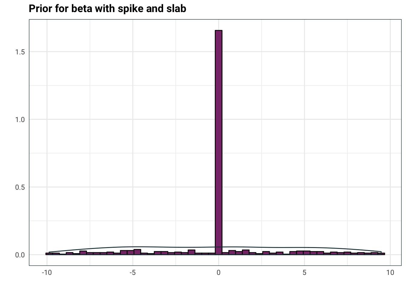
Now you can see where the slab comes from, it’s what the prior for \(\beta\) looks like when it’s non-zero. Above, I used \(\Gamma^{-1}(0.1, 0.1)\) but typically you can crank down the parameters for an even slabbier slab, or use a half-Cauchy random variable.
OK, so last but not least is the pesky \(\Sigma'\). You can, of course, set it to identity, or even better, set it to your prior beliefs about the interactions between the \(\beta_i\) (the diagonal term is irrelevant, we only care about the interactions). This might be somewhat implausible if you have a lot features. In such case, one option is to use a Zellner prior and set \(\Sigma' = (X^T X)^{-1}\). That’s right, we are peaking into the data for our prior, which is known as empirical Bayes. To understand why we chose that \(\Sigma\), suppose we are doing frequentist linear regression for a second. The OLS solution is \(\hat \beta = (X^TX)^{-1} X^T y\) and since \(y~ N(X\beta, \sigma^2)\) we have that \[ \text{Var}(\hat\beta) = (X^TX)^{-1} X^T \sigma^2 [(X^TX)^{-1} X^T]^T = \sigma^2 (X^TX)^{-1}. \] Since we don’t care about the scaling of \(\Sigma\), setting it to be \((X^TX)^{-1}\) gives it the same covariance structure as the frequentist \(\hat \beta\), which we are saying is our prior assumption. Though there is one quirk here which is that \(X^TX\) might not be invertible, so we also just add the diagonal elements: \(\Sigma = [(1/2) X^TX + (1/2) \text{diag}(X^TX)]^{-1}\).
Since Stan does not support discrete parameters, here is an implementation in PyMC3:
import pymc3 as pm
import numpy as np
def get_model(y, X):
    model = pm.Model()
    Sigma = .5 * np.matmul(X.T, X)
    Sigma += np.diag(np.diag(Sigma))
    Sigma = np.linalg.inv(Sigma)
    with model:
        xi = pm.Bernoulli('xi', .5, shape=X.shape[1])
        tau = pm.HalfCauchy('tau', 1)
        sigma = pm.HalfNormal('sigma', 10)
        beta = pm.MvNormal('beta', 0, tau * Sigma, shape=X.shape[1])
        mean = pm.math.dot(X, xi * beta)
        y_obs = pm.Normal('y_obs', mean, sigma, observed=y)
    return model