Introduction to Hamiltonian Monte Carlo
One thing that has been occupying my head in the past couple of weeks has been HMC and how it can be used in large data/large model context. HMC stands for Hamiltonian Monte Carlo and it’s the de facto Bayesian method for sampling due to it’s speed. Before getting into big datasets and big models, let me motivate this problem a little bit.
If you are new to Bayesian modelling, I have a little primer on the topic so I will assume for the most part you are familiar with basic Bayesianism. Let’s say we build our cute model by constructing a likelihood $p(y|x, \theta)$ and prior $p(\theta)$, then to obtain the posterior, we can use Bayes rule:
$$ p(\theta| x, y) = \frac{p(y | x, \theta)p(\theta)}{\int_\theta p(y | x, \theta)p(\theta)} $$
Now when we can work out the integral at the bottom analytically, all is well, we just plug it in and BAM, out comes the posterior. Unfortunately, this is a rather special case and more often than not, we don’t know what that integral is. We usually know the posterior up to a constant:
$$ p(\theta| x, y) \propto f(\theta) = p(y | x, \theta)p(\theta) $$
If you are from the machine learning crowd, you can think of this $f$ as taking in as the input the weights of the neural network and outputting the loss of the neural network with those weights on your whole data.
Sampling is hard
First thing almost everyone learns in undergraduate maths is the trapezoid rule for estimating the integral. Basically, you take equally spaced points in your space, evaluate the function at those points and multiply by some volume factor. To achieve an error rate of $\epsilon$, you are going to need $O(\epsilon^{-2p})$ number of points. Let’s put some real numbers here, suppose we want an error rate of 0.01 for say ResNet-152 which has 60m parameters. This would require roughly $10^{200,000,000}$ points to evaluate. Just to put this into perspective, there is an estimate number of $10^{80}$ atoms in the observable universe!
Enter in Markov chain Monte Carlo
Markov chain Monte Carlo is a simple idea: you build a Markov chain, which has its invariant measure $p(\theta| x, y)$, then with some regularity assumptions you get that the chain converges to this distribution.
For convenience, let’s just call our measure of interest $\pi(\theta) = p(\theta| x, y)$ and remember that we can only compute this up to some unknown constant with $f(\theta)$. We can specify a Markov chain by its transition probabilities $K(\theta' | \theta)$ which notes the probability of moving to state $\theta'$ when we are in state $\theta$. The detailed balance equations state the Markov chain with transition probabilities $K$ has a unique stationary distribution $\pi$ if
$$ \pi(\theta) K(\theta' | \theta) = \pi(\theta') K(\theta | \theta'). $$
Under certain regularity assumptions we can also show that the Markov chain converges to this stationary distribution as time tends to infinity.
So how can we construct a Markov chain with $\pi$ as the stationary measure when we only know it up to a constant?
There is an easy way of doing this using the Metrapolis Hastings algorithm. The idea is given we are at $x$, we are going to propose a new location $x'$ using the pdf $\zeta(x'| x)$. Then you build a Markov chain like this:
- Given $X_t$ we move as follows.
- Sample $\xi_t$ from $\zeta(\cdot | X_t)$.
- Set the acceptance probability to be \[ a_t := \min\left\{1, \frac{f(\xi_{t})\zeta(X_t| \xi_t)}{f(X_t)\zeta(\xi_t| X_t)}\right\} \]
then the transition to the next step is given by
\[ X_{t+1} = \begin{cases} \xi_t & \text{with probability } a_t \\ X_{t} & \text{with probability }1 - a_t \end{cases} \]
In words, we have a proposal $\xi_t$ for each step. If the proposal $\xi_{t}$ has a high enough probability compared to $X_{t}$, we accept it, otherwise we reject the proposal.
Writing out the transition probabilities, you can see easily that they satisfy the detailed balance equation because $\frac{f(\xi_{t})}{f(X_t)}=\frac{\pi(\xi_{t})}{\pi(X_t)}$.
The most obvious proposal distribution is given by a normal distribution: $$ \zeta(x'| x) = \frac{1}{(2\pi)^{d/2}} e^{-\frac{1}{2}(x' - x)^T (x' - x)} $$ and for this distribution we have a key properly which is $\zeta(x'| x) = \zeta(x| x')$ so that the acceptance probability is just the ratio of the proposed points.
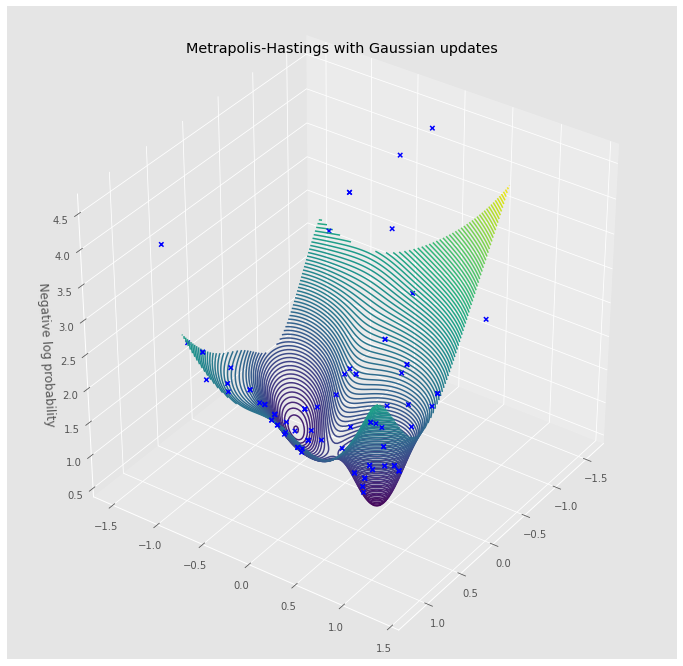
In the implementation below, I have worked with the negative log densities, e.g. $-\log \pi$ which is called surface. Generally it’s easier to do the computations above in log land and it will become even more so when we look at Hamiltonian Monte Carlo.
import numpy as np
from torch.distributions import MultivariateNormal
import matplotlib.pyplot as plt
import torch
plt.style.use('ggplot')

def generate_cov(state):
    corr = state.uniform()
    cov = state.uniform(0, 0.5) * np.array([[1, corr], [corr, 1]])
    return cov

class TestSurface(object):
    def __init__(self, n=10):
        self.n = n
        state = np.random.RandomState(2021)
        self.rvs = [
            MultivariateNormal(
                torch.tensor(state.uniform(-1, 1, size=(2))),
                torch.tensor(generate_cov(state))
            )
            for _ in range(n)
        ]

    def __call__(self, x):
        output = 0.0
        for rv in self.rvs:
            output += torch.exp(rv.log_prob(x)) / self.n
        return -torch.log(output)
class GaussianMH(object):
    def __init__(self, surface, scale=0.5):
        self.surface = surface
        self.scale = scale
        self.state = np.random.RandomState(1234)

    def step(self, x=None):
        if x is None:
            x = np.array([0.0, 0.0])
        sample = self.state.normal(size=2, scale=self.scale)
        proposal = x + sample
        if self.is_accepted(x, proposal):
            return proposal
        return x

    def is_accepted(self, x_old, x_new):
        new_log_pba = - self.surface(torch.tensor(x_new))
        old_log_pba = - self.surface(torch.tensor(x_old))
        with torch.no_grad():
            accept_pba = (new_log_pba - old_log_pba).exp().detach().numpy()
        if accept_pba > 1:
            return True
        if self.state.rand(1) < accept_pba:
            return True
        return False

surface = TestSurface(15)

mh = GaussianMH(surface)
walk = [mh.step()]
for _ in range(100):
    walk.append(mh.step(walk[-1]))
walk = np.stack(walk, axis=0)

fig = plt.figure(figsize=(12, 12))
ax = plt.axes(projection='3d')
x = np.linspace(-1, 1, 100)
y = np.linspace(-1, 1, 100)
X, Y = np.meshgrid(x, y)
input = torch.tensor(np.stack([X.reshape(-1), Y.reshape(-1)], axis=1))
Z = surface(input).numpy().reshape(*X.shape)

ax.scatter(walk[:, 0], walk[:, 1],
           surface(torch.tensor(walk)).numpy(),
           marker='x', c='blue', alpha=1.0, label='Accepted')
ax.contour3D(X, Y, Z, 100)
ax.view_init(35, 35)
ax.set_xlabel('')
ax.set_ylabel('')
ax.set_zlabel('Negative log probability')
ax.set_title('Metrapolis-Hastings with Gaussian updates')
fig.show()
Hamiltonian Monte Carlo
Metropolis-Hastings algorithm with Gaussian updates do not scale well to high dimensions. The reason for this is because in high dimensions, the probability that selecting a random point has a high enough density is pretty low and just gets lower as we increase the dimension. So in high dimensions, it’s essential to make sure we propose points in a way that respects the density we are trying to sample from.

The idea of the Hamiltonian Monte Carlo is to introduce an auxiliary variable and sample jointly from this bigger space. For this, we look at the space $(\theta, r) \in \mathbb{R}^{d + d}$ where $r \in \mathbb{R}^d$ is called the momentum (we will see why in a bit). Next the joint density on this space is given by:
$$ q(\theta, r) = \pi(\theta) \mathcal N(r| 0, \Sigma) \propto f(\theta) \mathcal N(r| 0, \Sigma) $$ where $\Sigma$ is a parameter which we can pick. In words, the measure $q$ is the product of two independent random variables, $\pi$ on the $\theta$ part and a normal random variable on the momentum part.
For convenience, let: $$ U(\theta) = -\log f(\theta) \qquad K(r) = -\log \mathcal N(r| 0, \Sigma) $$ so that $$ q(\theta, r) = \frac{1}{Z}e^{-U(\theta)} e^{-K(r)}. $$
Now imagine that we have a ball at position $\theta$ with momentum $r$, then we make this ball move on the log density $U$ by using Hamiltonian dynamics: \[ \begin{aligned} \frac{d\theta}{dt} & = \frac{dK}{dr} \\ \frac{dr}{dt} & = \frac{dU}{d\theta} \end{aligned} \]
Let’s refer to the solution at time $t$ by $(\theta_t, r_t)$ from some initial point. The really cool thing about the Hamiltonian dynamics is that it retains the same density throughout: $$ q(\theta_t, r_t) = q(\theta_{t'}, r_{t'}) \qquad \forall , t, t' >0 $$
OK, so now we are set to describe how we can use this. First, we are going to sample from the joint density $q$, after which, we can just ignore $r$ samples which will result in samples from $\pi$. We can use the deterministic proposal like this: $$ \zeta(\theta', r' | \theta, r) = \delta_{\text{H}_t(\theta, r)}(\theta', -r') $$ where $\text{H}_t$ is the Hamiltonian dynamics applied for time $t>0$ (which is a parameter we can adjust). So in this case, our proposal is deterministic.
Why do we have $-r'$ in the equation above? Well if you look closely at the dynamics, you will realise that if $(\theta_t, r_t) = \text{H}_t(\theta, r)$, then $(\theta, r) = \text{H}_t(\theta_t, -r_t)$, so adding the minus sign gives us reversibility. Because the Hamiltonian dynamics gives us a point with the same probability as the starting point, this means the Metropolis-Hastings acceptance ratio is always 1, i.e. we always accept the proposal generated in this form. This means that this transition leaves the measure $q$ invariant.
Instead of applying Metropolis-Hastings updates repeatedly, we can utilise an other trick. The reason for this trick is to reduce the autocorrelation of the samples, because remember Metropolis-Hastings guarantees that samples are from the target distribution, but they might be very correlated, which is obviously not ideal. To do this, we can just sample the momentum variable $r$ at each step. To conclude, the HMC algorithm is:
- Sample $r \sim N(0, \Sigma)$ where $\Sigma$ is a parameter that the user selects.
- Run Hamiltonian dynamics for time t and record the resulting $\theta_t$.
Since both of those steps leave the measure $q$ invariant we are guaranteed under regularity assumptions to sample from the measure $\pi$ as we run more steps.
Finally there is a final step. In practice we can’t simulate the Hamiltonian dynamics exactly. In the example below, I have used the Leapfrog method for this. This means that our proposed state will have some degree of error and thus will not quite have the same density under $q$. This means in practice we have to run a Metropolis-Hastings proposal step with the proposal at the end:
- Work out the acceptance probability \[ a_t = \min\left\{1, \frac{f(\theta_t)}{f(\theta)}\right\} \] and accept the sample with probability $a_t$.
from tqdm.autonotebook import tqdm
class HMC(object):
def __init__(self, surface, step_size=1e-4, path_length=100):
self.surface = surface
self.step_size = step_size
self.path_length = path_length
self.state = np.random.RandomState(1234)
def step(self, x=None, momentum=None):
if momentum is None:
momentum = torch.tensor(self.state.normal(size=2))
if x is None:
x = torch.tensor([0.0, 0.0])
x.requires_grad_(True)
# Leap-frog method on numerically solving the Hamiltonian eq
point = self.surface(x)
point.backward()
with torch.no_grad():
momentum = momentum - 0.5 * self.step_size * x.grad
x += self.step_size * momentum
point = self.surface(x)
point.backward()
with torch.no_grad():
momentum = momentum - 0.5 * self.step_size * x.grad
x.requires_grad_(False)
return x.detach(), momentum.detach()
def _calculate_hamiltonian(self, x, momentum):
with torch.no_grad():
# Negative log density of normal up to constant
momentum_term = (momentum ** 2).sum()
x_term = self.surface(x)
return x_term + momentum_term
def is_accepted(self, x_old, x_new, momentum_old, momentum_new):
accept_pba = (
self._calculate_hamiltonian(x_old, momentum_old) -
self._calculate_hamiltonian(x_new, momentum_new)
).exp()
if accept_pba > 1:
return True
if torch.rand(1) < accept_pba:
return True
return False
def walk(self, x=None, momentum=None):
x, momentum = self.step(x=x, momentum=momentum)
for _ in range(self.path_length - 1):
x, momentum = self.step(x=x, momentum=momentum)
return x, momentum
hmc = HMC(surface, step_size=0.1, path_length=10)
walks = []
is_accepted = []
x = torch.tensor([0.0, 0.0])
momentum = torch.tensor(hmc.state.normal(size=2))
for _ in tqdm(range(100)):
x_new, momentum_new = hmc.walk(x=x, momentum=momentum)
is_accepted.append(hmc.is_accepted(x, x_new, momentum, momentum_new))
walks.append(np.copy(x_new.detach().numpy()))
x = x_new
momentum = torch.tensor(hmc.state.normal(size=2))
walks = np.stack(walks, axis=0)
is_accepted = np.array(is_accepted)
fig = plt.figure(figsize=(12, 12))
ax = plt.axes(projection='3d')
x = np.linspace(-2, 2, 100)
y = np.linspace(-2, 2, 100)
X, Y = np.meshgrid(x, y)
input = torch.tensor(np.stack([X.reshape(-1), Y.reshape(-1)], axis=1))
Z = surface(input).numpy().reshape(*X.shape)
accepted_walk = walks[is_accepted, :]
rejected_walk = walks[~is_accepted, :]
ax.scatter(accepted_walk[:, 0], accepted_walk[:, 1],
surface(torch.tensor(accepted_walk)).numpy(),
marker='x', c='blue', alpha=1.0, label='Accepted')
ax.scatter(rejected_walk[:, 0], rejected_walk[:, 1],
surface(torch.tensor(rejected_walk)).numpy(),
marker='x', c='red', alpha=1.0, label='Rejected')
ax.contour3D(X, Y, Z, 100)
ax.view_init(45, 20)
ax.set_xlabel('x')
ax.set_ylabel('y')
ax.set_zlabel('z')
ax.legend()
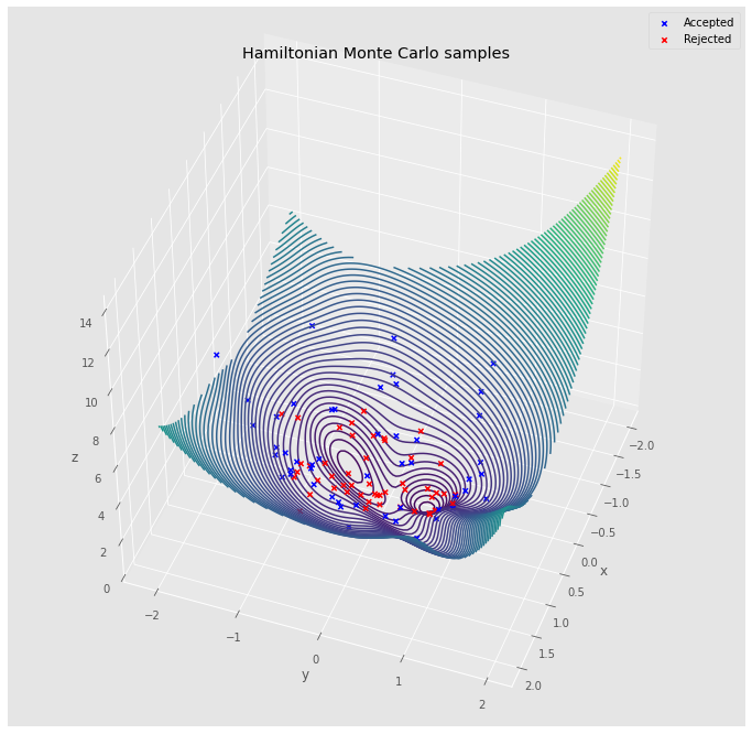
ax.set_title('Hamiltonian Monte Carlo samples')
fig.show()
Where to from here?
HMC is a great way to sample in high dimensions because the acceptance probability is going to be very close $1$ (it’s the error between the discrete ODE vs continuous ODE). This makes it a really nice tool. I have below some further materials if you would like to get a deeper dive into HMC.
- Excellent survey of HMC by Michael Betancourt
- No U Turn Sampling (NUTS) is the state of the art in HMC method
- Stan’s reference manual on HMC
- Great paper about how we can practically measure if the MCMC chain is sampling well (remember that the guarantees are all asymptotic and we only have finite time!)