Variational auto-encoders (VAEs) are a latent space model. The idea is you have some latent space variable $z \in \mathbb{R}^{k}$ which describes your original variables $x\in\mathbb{R}^d$ in higher dimensional space by a latent model $p(x|z)$. Let’s assume that this distribution is given by a neural network with some parameters $\theta$ so that we assume $$ x | z, \theta \sim N(g_\theta(z), 1). $$ Of course in reality, we don’t know $(z, \theta)$, we would like to infer these from the data. Bayes to the rescue: $$ z, \theta | x = \frac{1}{Z} p(z)p(\theta) p(x|z) $$ where $Z$ is a normalisation constant.
The problem with Bayesian inference is that the constant $Z$ is quite difficult to work out. One approach is to use variational inference, meaning, we use some parametric distribution $q_\phi$ to approximate $p(z,\theta|x)$ by minimising some distance on probability distributions: $$ (\hat\phi, \hat\theta) = \text{argmin}_{(\phi, \theta)} D\Big(q_\phi(\cdot), p(\cdot, \theta | x)\Big). $$
A primer on Wasserstein distance
There are quite few choices we can make for $D$, the distance on probability measures. The only restriction here is we know $p(z, \theta | x)$ up to a constant. Using Kullback–Leibler divergence, we get the ELBO lower bound to optimise.
Alternatively, we can use Wasserstein metric which is given by $$ D(q, p) = W_p(q, p)= \inf_{\Gamma} \mathbb{E}_{(X, Y) \sim \Gamma}\Big[\|X - Y\|^p_p\Big]^{\frac{1}{p}} $$ where the infimum is taken over all couplings of $q$ and $p$.
It’s worth thinking about how this works. A coupling of two random variables is putting them in the same probability space so that the marginals are given by the respective distributions. So as an example, lets say the two random variables are $N(0.5, 1)$ and $N(0, 1)$ and $p=1$. How might we go about constructing this coupling? Here are two examples of couplings:
-
Sample $X \sim N(0.5, 1)$ and take $Y \sim N(0, 1)$ independently. In this case $E[(X-Y)^2]=0.5 ^2 + 1=1.25$, since the difference is just a normal random variable.
-
Sample $X \sim N(0.5, 1)$ and take $Y = X - 0.5$. In this case $E[(X-Y)^2] = 0.5^2 =0.25$.
We can see that $W_2(q,p) \leq 0.5$ (taking square roots of the above calculation) since 2) is a better bound.
When $p=1$, the Wasserstein metric has a nice dual representation: $$ W_1(p, q) = \sup_{f \text{ 1-Lipschitz}}\mathbb E_{X\sim p}[f(X)] - \mathbb E_{Y \sim q}[f(Y)]. $$ This duality is really nice in practice, because mathematically we can upper bound $W_1$ using couplings, and lower bound by using the above formula. Back to the above example with $N(0.5, 1)$ and $N(0, 1)$, the coupling in 2) above shows that the $W_1$-distance is at most $0.5$. On the other hand if we just take $f$ to be the identity we can see that $$ W_1(p,q) \geq \mathbb E_{X\sim p}[X] - \mathbb E_{Y \sim q}[Y] = 0.5 $$ and thus $W_1$-distance is infact exactly $0.5$.
So what’s the difference to KL?
The KL-distance has a few undesirable properties, especially when the support of the distributions do not match. Consider the case on $\mathbb{R}^2$, lets take $p$ to be uniformly distributed on ${0}\times[0,1]$ and $q$ uniformly distributed on ${0.1}\times[0,1]$. In this case $W_1(p,q)=0.1$, which makes the them look close. On the other hand $$ \text{D}_{KL}(p||q) = \int p(x) \log\left(\frac{p(x)}{q(x)}\right) dx = \infty $$ and similrly $\text{D}_{KL}(q||p) = \infty$, which is not very desirable.
Wasserstein and neural networks
Wasserstein GANs minimise the $W_1$. The original paper suggested taking a feed-forward network $h_\psi$ and clipping the weights $\psi$ to be in some range. Secondary paper instead the objective for $\phi$ to be $$ \text{argmin}_{\psi} \mathbb E_{X\sim p}[h_\psi(X)] - \mathbb E_{Y \sim q}[h_\psi(Y)] + \lambda \Big(\|\nabla_\psi h_\psi\|_2 - 1\Big)^2 $$ so that the gradient of the resulting network should roughly be around $1$.
That side note aside, what I really want to discuss here is Wasserstein autoencoders. In this paper it is assumed that the generative model $q(x|z)$ is not random i.e. there exists a function $g$ and set of parameters $\theta$ such that $$ q(x | z) = \delta_{g_\theta(z)}(x) $$ which simplifies the situation a lot more. This is going to get a little bit confusing so let’s say that the prior on the latent space is $q_Z$, the marginal of the model on $X$ is $q_X$ and the true distribution of the data is $p_X$, which is unknown to us. Then $$ W_p(p_X, q_X)^p = \inf_{(X, Y)\sim \Gamma}\mathbb E[\|X - Y\|_p^p] = \inf_{(X, Z)\sim \Gamma}\mathbb E[\|X - g_\theta(Z)\|_p^p]. $$ Now if $\gamma$ denotes a coupling between $X$ and $Z$, we can always write this as $\gamma(x) \gamma(z|x) = p_X(x)\gamma(z|x)$. Thus we can take the infimum over all $\tilde\gamma$: $$ W_p(p_X, q_X)^p = \inf_{\gamma: \int p_X(x)\gamma(\cdot|x)dx = q(\cdot)}\mathbb E_{p_X}\mathbb E_{\gamma(\cdot|x)}[\|X - g_\theta(Z)\|_p^p]. $$ The paper then relaxes this constrained optimsation by taking a metric on probability measures $D$ and setting the objective as $$ \text{argmin}_{\gamma, \theta} \mathbb E_{p_X}\mathbb E_{\gamma(\cdot|x)}[\|X - g_\theta(Z)\|_p^p] + \lambda D(q_Z, \gamma). $$ If you squint close enough, you can see two neural networks to minimise the objective above.
-
The decoder $g_\theta$ which, given the latent representation maps to the feature space.
-
The encoder $\gamma(z|x)$ which maps the features to latent representations.
We can also get a third neural network in there as well! If we use the Jensen-Shannon distance when measuring the disparity $D(q_Z, \gamma)$, this results can be formulated using a neural network which acts as a distriminator (just like in plain old GANs).
This results in the algorithm:

I have a simple implementation here.
import tensorflow as tf
import matplotlib.pyplot as plt
%matplotlib inline
import seaborn as sns
import numpy as np
import pandas as pd
(x_train, y_train), (x_test, y_test) = tf.keras.datasets.mnist.load_data()
x_train = x_train.astype(np.float32) / 256
x_train = x_train[:, :, :, np.newaxis]
x_test = x_test.astype(np.float32) / 256
x_test = x_test[:, :, :, np.newaxis]
y_train = y_train.astype(np.int32)
y_test = y_test.astype(np.int32)
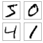
fig, axes = plt.subplots(figsize=(3, 3),
nrows=2,
ncols=2)
axes = axes.flatten()
for i, ax in enumerate(axes):
ax.imshow(x_train[i, :, :, 0], cmap='Greys')
ax.grid(False)
ax.set_xticks([])
ax.set_yticks([])
def model_fn(features, labels, params, mode):
    encoder = tf.keras.models.Sequential([
                tf.keras.layers.Conv2D(64, [2, 2], input_shape=(28, 28, 1),
                                       activation='linear'),
                tf.keras.layers.BatchNormalization(),
                tf.keras.layers.LeakyReLU(),
                tf.keras.layers.Conv2D(32, [3,3], activation='linear'),
                tf.keras.layers.BatchNormalization(),
                tf.keras.layers.LeakyReLU(),
                tf.keras.layers.Conv2D(32, [3,3], activation='linear'),
                tf.keras.layers.BatchNormalization(),
                tf.keras.layers.LeakyReLU(),
                tf.keras.layers.Flatten(),
                tf.keras.layers.Dense(32, activation='relu'),
                tf.keras.layers.Dense(16, activation='relu'),
                tf.keras.layers.Dense(8, activation='relu'),
                tf.keras.layers.Dense(params['latent_dim'],
                                      activation='linear'),
    ])
    decoder = tf.keras.models.Sequential([
          tf.keras.layers.Dense(units=7*7*32, activation=tf.nn.relu,
                                input_shape=(params['latent_dim'], )),
          tf.keras.layers.Reshape(target_shape=(7, 7, 32)),
          tf.keras.layers.Conv2DTranspose(
              filters=64,
              kernel_size=3,
              strides=(2, 2),
              padding="SAME",
              activation='relu'),
          tf.keras.layers.Conv2DTranspose(
              filters=32,
              kernel_size=3,
              strides=(2, 2),
              padding="SAME",
              activation='relu'),
          tf.keras.layers.Conv2DTranspose(
              filters=1, kernel_size=3, strides=(1, 1), padding="SAME"),
    ])
    discriminator = tf.keras.models.Sequential([
                tf.keras.layers.Dense(128, activation='relu',
                                      input_shape=(params['latent_dim'], )),
                tf.keras.layers.Dense(128, activation='relu'),
                tf.keras.layers.Dense(128, activation='relu'),
                tf.keras.layers.Dense(128, activation='relu'),
                tf.keras.layers.Dense(1, activation='sigmoid'),
    ])

    encoded = encoder(features)
    prior_samples = tf.random.normal(tf.shape(encoded), 0.0, 2.0)

    if mode == tf.estimator.ModeKeys.PREDICT:
        samples = decoder(prior_samples)
        return tf.estimator.EstimatorSpec(mode=mode,
                                          predictions={
                                              'encoding': encoded,
                                              'samples': samples,
                                              })


    prior_log_prob = tf.math.log(discriminator(prior_samples) + 1e-6)
    encoded_prob = discriminator(encoded)
    om_encoded_log_prob = tf.math.log(1 - encoded_prob + 1e-6)
    discrim_loss = -tf.reduce_mean(prior_log_prob + om_encoded_log_prob)
    discrim_loss *= params['lambda']
    tf.summary.scalar('disriminator', discrim_loss)

    decoded = decoder(encoded)
    vae_loss = tf.reduce_mean((features - decoded) ** 2)
    vae_loss -= tf.reduce_mean(tf.math.log(encoded_prob)) * params['lambda']
    tf.summary.scalar('variational_loss', vae_loss)
    total_loss = vae_loss + discrim_loss

    if mode == tf.estimator.ModeKeys.EVAL:
        return tf.estimator.EstimatorSpec(mode=mode,
                                          loss=total_loss,
                                          predictions={'encoding': encoded})
    discrim_optimiser = tf.train.AdamOptimizer(params['lr'])
    enc_dec_optimiser = tf.train.AdamOptimizer(params['lr'])
    discrim_op = discrim_optimiser.minimize(discrim_loss,
                                            var_list=discriminator.weights)
    enc_dec_op = enc_dec_optimiser.minimize(
                        vae_loss,
                        var_list=encoder.weights + decoder.weights,
                        global_step=tf.train.get_or_create_global_step(),
                        )
    train_op = tf.group([discrim_op, enc_dec_op])
    return tf.estimator.EstimatorSpec(mode=mode,
                                      loss=total_loss,
                                      predictions={'encoding': encoded},
                                      train_op=train_op)
def input_fn(params, mode):
    if mode == tf.estimator.ModeKeys.EVAL or \
       mode == tf.estimator.ModeKeys.PREDICT:
        dataset = tf.data.Dataset.from_tensor_slices(
            (x_test, y_test)
        )
    else:
        dataset = tf.data.Dataset.from_tensor_slices(
                (x_train, y_train)
            )
        dataset = dataset.shuffle(10000).repeat(params['epochs'])
    return dataset.batch(params['batch_size'])
params = {
    'lr': 8e-5,
    'lambda': 0.001,
    'epochs': 200,
    'batch_size': 218,
    'latent_dim': 1,
}

run_config = tf.estimator.RunConfig(model_dir='./wae',
                                    save_checkpoints_steps=1000)

estimator = tf.estimator.Estimator(model_fn,
                                   params=params,
                                   model_dir='./wae',
                                   config=run_config)

train_spec = tf.estimator.TrainSpec(input_fn=input_fn)
eval_spec = tf.estimator.EvalSpec(input_fn=input_fn)
tf.estimator.train_and_evaluate(estimator, train_spec, eval_spec)
estimator = tf.estimator.Estimator(model_fn,
params=params,
model_dir='./wae')
preds = estimator.predict(lambda : input_fn(params, tf.estimator.ModeKeys.EVAL))
preds = [(x['encoding'], x['samples']) for x in preds]
encoding = [x[0] for x in preds]
samples = [x[1] for x in preds]
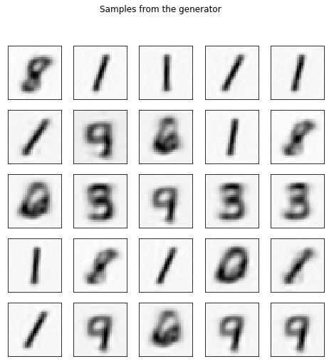
fig, axes = plt.subplots(figsize=(8, 8),
nrows=5,
ncols=5)
axes = axes.flatten()
for i, ax in enumerate(axes):
ax.imshow(samples[-i][:, :, 0], cmap='Greys')
ax.grid(False)
ax.set_xticks([])
ax.set_yticks([])
fig.suptitle('Samples from the generator')
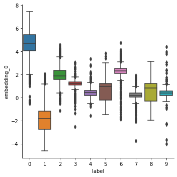
df = pd.DataFrame(np.stack(encoding, axis=0))
df.columns = [f'embedding_{i}' for i in range(df.shape[1])]
df['label'] = y_test.reshape(-1)
sns.catplot(data=df, y='embedding_0', x='label', kind='box')