There has been some really amazing advances in natural language processing (NLP) in the last couple of years. Back in November 2018, Google released https://ai.googleblog.com/2018/11/open-sourcing-bert-state-of-art-pre.html, which is based on attention mechanisms in Attention Is All You Need. In this two part series, I will assume you know nothing about NLP, have some understanding about neural networks, and take you from the start to end of understanding how transformers work.
Natural language processing is the art of using machine learning techniques in processing language. There are several goals one could have for this. For example, we could try to analyse sentiment from online reviews or translating sentences from one language to an other.

The first challenge here is that most machine learning techniques require vectors, i.e. numerical values, as input and output. So how do we do that with words? A very naive way of doing is to use one hot encoding. This maps each word to a series of zeros and ones like this:
import string
import pandas as pd
import numpy as np

sentence = 'How much wood would a woodchuck chuck if a woodchuck could chuck wood?'
def clean_sentence(s):
    s = s.lower()
    translator = s.maketrans('', '', string.punctuation)
    return s.translate(translator)
cleaned = clean_sentence(sentence)
print(f'Original: {sentence}\nCleaned: {cleaned}')

words = set(cleaned.split(' '))

def zero_one(i, n_words):
    vec = np.zeros(n_words)
    vec[i] = 1
    return vec

def make_numeric(words):
    n_words = len(words)
    return {word: zero_one(i, n_words) for i, word in enumerate(words)}

simple_numeric = make_numeric(words)
X = pd.DataFrame(
    np.array([simple_numeric[w] for w in cleaned.split(' ')]),
    index=cleaned.split(' '),
    columns=words)
X
Original: How much wood would a woodchuck chuck if a woodchuck could chuck wood?
Cleaned: how much wood would a woodchuck chuck if a woodchuck could chuck wood
| would | much | how | wood | woodchuck | could | chuck | if | a | |
|---|---|---|---|---|---|---|---|---|---|
| how | 0.0 | 0.0 | 1.0 | 0.0 | 0.0 | 0.0 | 0.0 | 0.0 | 0.0 |
| much | 0.0 | 1.0 | 0.0 | 0.0 | 0.0 | 0.0 | 0.0 | 0.0 | 0.0 |
| wood | 0.0 | 0.0 | 0.0 | 1.0 | 0.0 | 0.0 | 0.0 | 0.0 | 0.0 |
| would | 1.0 | 0.0 | 0.0 | 0.0 | 0.0 | 0.0 | 0.0 | 0.0 | 0.0 |
| a | 0.0 | 0.0 | 0.0 | 0.0 | 0.0 | 0.0 | 0.0 | 0.0 | 1.0 |
| woodchuck | 0.0 | 0.0 | 0.0 | 0.0 | 1.0 | 0.0 | 0.0 | 0.0 | 0.0 |
| chuck | 0.0 | 0.0 | 0.0 | 0.0 | 0.0 | 0.0 | 1.0 | 0.0 | 0.0 |
| if | 0.0 | 0.0 | 0.0 | 0.0 | 0.0 | 0.0 | 0.0 | 1.0 | 0.0 |
| a | 0.0 | 0.0 | 0.0 | 0.0 | 0.0 | 0.0 | 0.0 | 0.0 | 1.0 |
| woodchuck | 0.0 | 0.0 | 0.0 | 0.0 | 1.0 | 0.0 | 0.0 | 0.0 | 0.0 |
| could | 0.0 | 0.0 | 0.0 | 0.0 | 0.0 | 1.0 | 0.0 | 0.0 | 0.0 |
| chuck | 0.0 | 0.0 | 0.0 | 0.0 | 0.0 | 0.0 | 1.0 | 0.0 | 0.0 |
| wood | 0.0 | 0.0 | 0.0 | 1.0 | 0.0 | 0.0 | 0.0 | 0.0 | 0.0 |
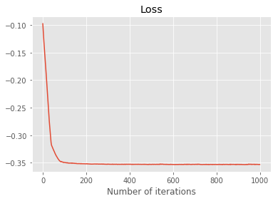
I have encoded the sentence to run down the columns so that each row corresponds to a word embedding. Although this expresses the words as numbers, it doesn’t really have any other information. In order to be able to extract some information, we need to make the embedding learn-able. The simplest way to do this is just to multiply by a matrix, where the matrix we multiply by can be optimized for. For example, we can train the model to embed words that appear in the same document closer together. The code below does exactly that, if $f$ is the embedding function then $$ \text{loss}_w =\sum_{v \in \text{Words}: v,w \text{ not in same sentence}} \frac{|f(w)f(v)|}{|f(w)|_2 |f(v)|_2} -\sum_{v \in \text{Words}: v,w \text{ in same sentence}} \frac{|f(w)f(v)|}{|f(w)|_2 |f(v)|_2} $$
import torch
torch.manual_seed(1234)
from torch import nn
from tqdm import tqdm

sentences = ['dogs are awesome',
             'animals are awesome',
             'dogs are cute',
             'cats really suck',
             'dogs and cats are animals']

stopwrds = ['and', 'are']

def split_no_stopwords(x):
    result = x.split(' ')
    return [x for x in result if x not in stopwrds]
words = set().union(*[split_no_stopwords(x) for x in sentences])
simple_numeric = make_numeric(words)
sentence_emb = {x: np.array([simple_numeric[w] for w in split_no_stopwords(x)])
                for x in sentences}

class SimpleEmbedding(nn.Module):
    def __init__(self, n_words, embedding_dim):
        super().__init__()
        matrix = torch.randn((n_words, embedding_dim))
        self.matrix = nn.Parameter(matrix)
    def forward(self, x):
        return x @ self.matrix

simple_embedding = SimpleEmbedding(len(words), 5)

def together(w1, w2):
    return max([w1 in x and w2 in x for x in sentences])
in_same = np.array(
    [[together(w1, w2) for w1 in words] for w2 in words],
    dtype=float
)
in_same = torch.Tensor(in_same)
X = torch.Tensor(np.array([simple_numeric[w] for w in words]))

optimiser = torch.optim.Adam(simple_embedding.parameters(),
                            lr=1e-2)
epochs = 1000
losses = list()
with tqdm(total=epochs) as tq:
    for _ in range(epochs):
        embed = simple_embedding(torch.Tensor(X))
        normed = torch.nn.functional.normalize(embed, p=2, dim=1)
        cosine = torch.abs(normed @ normed.transpose(0,1))
        loss = -torch.mean(cosine * in_same)
        loss += torch.mean(cosine * (1-in_same))
        losses.append(loss.detach().numpy())
        loss.backward()
        optimiser.step()
        optimiser.zero_grad()
        tq.update(1)
        tq.set_description('loss: {:.2f}'.format(loss))
loss: -0.35: 100%|██████████| 1000/1000 [00:05<00:00, 169.89it/s]
import matplotlib.pyplot as plt
plt.style.use('ggplot')
%matplotlib inline
plt.plot(losses)
plt.title('Loss')
plt.xlabel('Number of iterations')
Text(0.5,0,'Number of iterations')
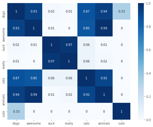
import seaborn as sns
df = pd.DataFrame(np.round(cosine.detach().numpy(), 2), index=words, columns=words)
fig, ax = plt.subplots(figsize=(9, 7))
sns.heatmap(df, annot=True, ax=ax, cmap='Blues')
<matplotlib.axes._subplots.AxesSubplot at 0x1a263235f8>
Just as a side node, pytorch and tensorflow (and probably other libraries but I only know these two) have ready made embedding modules. These do exactly the same as above but with a key speed improvement. I didn’t really need to multiply the one hot encoded matrix by the encoding matrix, I can just look up the word by the row it’s in, which is what these layers do.
Now let’s start thinking about how we might translate from one language to an other. Context really matters, the word stick has a completely different meaning in the sentence -my dog fetched a stick at the park- and -I’m going to stick with my phone plan, please stop calling me, I swear this is like th 10th time this week, I mean it’s just getting…- Sorry, got a bit side tracked there. The embedding we discussed so far would not be able to distinguish them. Even if we just ignored grammar, we can’t get away with just mapping words to words, instead what we need is map $f: \text{words}\times\text{context}\to\text{words}\times\text{context}$.

Attention mechanisms are a convenient way of expressing a relationship between the words in a sentence. For example let’s imagine we are looking at the sentence my dog is old, it likes to sleep. Attention mechanism picks up the words one by one and assigns a context to them. Imagine we are looking at the word it. You might think the context for that word looks like this:
my dog is old, it likes to sleep
Attention mechanism does this by creating a query, key and value vectors for each word. These are obtained by taking the words embedding and multiplying it by a matrix that is optimised for: $$ \begin{aligned} K_w = \text{embedding}(w) \cdot W_K, \quad W_K \in \mathbb{R}^{d_{\text{embedding}}, d_K} \\Q_w = \text{embedding}(w) \cdot W_Q, \quad W_Q \in \mathbb{R}^{d_{\text{embedding}}, d_K}\\V_w = \text{embedding}(w) \cdot V_K, \quad V_K \in \mathbb{R}^{d_{\text{embedding}}, d_V}. \end{aligned} $$ These matricies are shared across words and the query and key are of the same length. Then while evaluating w, the context of w is given by $$ \sum_{v\in \text{words}}\text{Attention}(Q_w, K_v, V_v) $$ where $$ \text{Attention}(Q_w, K_v, V_v) = \frac{exp\left(\frac{Q_w^t K_v}{\sqrt(d_K)}\right)}{\sum_{u \in \text{words}}exp\left(\frac{Q_w^t K_u}{\sqrt(d_K)}\right)} V_v. $$ The formula above looks a bit scary, but is a bit easier when it’s written in matrix form if we stack the query, keys and values in matricies where each row corresponds to a word $$ \text{Attention}(Q, K, V) = \text{softmax}\left(\frac{QK^t}{\sqrt d_k}\right) V $$ The scaling by the sqrt size of the dimension is used to counteract vanishing gradients.
With the machine learning philosophy of, if it ain’t broke, keep doing it, we could make several attention matricies and concatinate them together. This is called multi-head attention. Here is an implementation:
from IPython.display import display
class Attention(nn.Module):
    def __init__(self, embed_dim, d_k, d_v):
        super().__init__()
        self.W_K = nn.Parameter(torch.randn((embed_dim, d_k)))
        self.W_Q = nn.Parameter(torch.randn((embed_dim, d_k)))
        self.W_V = nn.Parameter(torch.randn((embed_dim, d_k)))
        self.scaling = torch.Tensor(np.array(1 / np.sqrt(d_k)))
    def _weight_value(self, x):
        K = x @ self.W_K
        Q = x @ self.W_Q
        V = x @ self.W_V
        weight = self.scaling * Q @ K.transpose(0, 1)
        exp_weight = torch.exp(torch.clamp(weight, max=25)) * mask
        attn = exp_weight / torch.sum(exp_weight,dim=1,keepdim=True)
        return attn, V
    def forward(self, x):
        weight, V = self._weight_value(x)
        return weight @ V

class MultiHeadAttention(nn.Module):
    def __init__(self, embed_dim, d_k, d_v, num_heads):
        super().__init__()
        self.attns = [Attention(embed_dim, d_k, d_v) for _ in range(num_heads)]
    def forward(self, x):
        results = [attn(x) for attn in self.attns]
        return torch.cat(results, dim=1)

embedding_dim = 10
embed = nn.Embedding(len(words), embedding_dim)
attention = Attention(10, 2, 2)
multi_attention = MultiHeadAttention(10, 2, 2, 3)

sentence = 'dogs are awesome'
words = set(sentence.split(' '))
numeric_encoder = {w: i for i, w in enumerate(words)}
sentence_num = np.array([numeric_encoder[w] for w in sentence.split(' ')])

emb = embed(torch.LongTensor(sentence_num))
attn = attention(emb)
multi_attn = multi_attention(emb)
def prettify(tensor):
    frame = pd.DataFrame(tensor.detach().numpy(), index=sentence.split(' '))
    return frame

print(f'Sentence: {sentence}\n')
print(f'Embedding:')
display(prettify(emb))
print('\n')
print(f'Attention:')
display(prettify(attn), )
print('\n')
print(f'Multi-head attention:')
display(prettify(multi_attn))
print('\n')
Sentence: dogs are awesome

Embedding:
| 0 | 1 | 2 | 3 | 4 | 5 | 6 | 7 | 8 | 9 | |
|---|---|---|---|---|---|---|---|---|---|---|
| dogs | -1.659277 | -1.877329 | 0.737246 | 0.391020 | 0.515788 | -1.004248 | -0.073698 | 0.314678 | -1.036901 | 0.210042 |
| are | -2.014255 | -1.517266 | 0.387743 | -1.184855 | 0.689674 | -0.283332 | -0.565951 | 0.356618 | 0.724366 | 0.032311 |
| awesome | 0.614427 | -0.055194 | -0.612545 | 0.750012 | 0.872818 | 0.766965 | -0.113781 | -0.942819 | 0.754022 | 0.136490 |
Attention:
| 0 | 1 | |
|---|---|---|
| dogs | 4.462710 | 4.086356 |
| are | 4.765477 | 4.637449 |
| awesome | 1.454956 | -0.845308 |
Multi-head attention:
| 0 | 1 | 2 | 3 | 4 | 5 | |
|---|---|---|---|---|---|---|
| dogs | 1.120507 | 2.196709 | 2.994548 | -2.731959 | -2.012827 | 2.491652 |
| are | -0.337405 | 0.715609 | 1.589315 | -2.042628 | -0.010207 | 0.305907 |
| awesome | 1.196454 | 2.192298 | 0.552418 | -0.452832 | 0.462553 | 4.359717 |
So OK, now we have the models, how do we actually set up a loss function and optimise for the parameters? What I have described above applies equally to images as well. For example Show and Tell: A Neural Image Caption Generator has some awesome plots on how attention mechanisms are used to generate image captions.
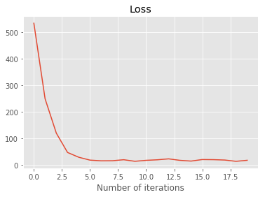
At this point, we will now hone in transformers for text translation. As a first step, we can train this model on trying to predict the next word in the sentence and see how it attributes attention. We will feed the words into the model one by one and ask it to predict the next word based off the past words it has seen.
from random import shuffle
class NextWordPredict(nn.Module):
    def __init__(self, n_words, n_embed):
        super().__init__()
        self.embedding = nn.Embedding(n_words, n_embed, )
        self.multi_attn = MultiHeadAttention(n_embed, n_embed // 4, n_embed // 4, 4)
        self.linear = nn.Linear(n_embed, n_words)
    def forward(self, x):
        emb = self.embedding(x)
        attn = self.multi_attn(emb)
        lin = self.linear(attn[-1, :])
        return torch.softmax(lin, dim=0)

buffet_quotes = """
I tell students to go work for an organization you admire or an individual you \
admire, which usually means that most MBAs I meet become self-employed.

Only when the tide goes out do you discover who has been swimming naked.

When you combine ignorance and leverage, you get some pretty interesting results.
"""
sentences = [clean_sentence(x.strip()) for x in buffet_quotes.split('.')[:-1]]
words = set().union(*[x.split(' ') for x in sentences])
n_words = len(words)
numeric_encoder = {w: i for i, w in enumerate(words)}
numerics = [np.array([numeric_encoder[w] for w in sent.split(' ')])
            for sent in sentences]

def one_hot(vec):
    if not isinstance(vec, np.ndarray):
        vec = np.array([vec])
    result = np.zeros((len(vec), n_words))
    for i, v in enumerate(vec):
        result[i, v] = 1.0
    return torch.Tensor(result)

epochs = 20
losses = list()
model = NextWordPredict(n_words, 100)
def loss_fun(y_pred, y_true):
    return -torch.sum(y_true * torch.log(y_pred))
optimiser = torch.optim.Adam(model.parameters(),
                             lr=1e-3)
numerics_ = list(numerics)
with tqdm(total=epochs) as tq:
    for _ in range(epochs):
        epoch_loss = 0
        shuffle(numerics_)
        for X in numerics_:
            for t in range(1, len(X) - 1):
                x_train = torch.LongTensor(X[:t])
                y_true = one_hot(X[t])
                y_pred = model(x_train)
                loss = loss_fun(y_pred, y_true)
                loss.backward()
                optimiser.step()
                optimiser.zero_grad()
                epoch_loss += loss.detach().numpy()
        losses.append(epoch_loss)
        tq.update(1)
        tq.set_description('loss: {:.2f}'.format(epoch_loss))
plt.plot(losses)
plt.title('Loss')
plt.xlabel('Number of iterations')
loss: 16.93: 100%|██████████| 20/20 [00:03<00:00,  4.37it/s]


Text(0.5,0,'Number of iterations')
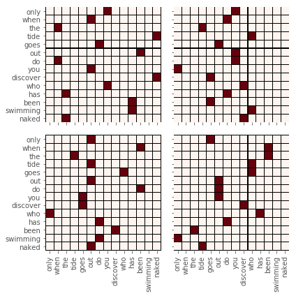
ex_num = numerics[1]
ex_sentence = sentences[1]
emb = model.embedding(torch.LongTensor(ex_num))
fig, ax = plt.subplots(figsize=(3 *2, 3 * 2),
                       nrows=2,
                       ncols=2,
                       sharex=True,
                       sharey=True)
ax = ax.flat
for i in range(4):
    weight_, _ = model.multi_attn.attns[i]._weight_value(emb)
    weight = weight_.detach().numpy()
    df = pd.DataFrame(weight, index=ex_sentence.split(' '), columns=ex_sentence.split(' '))
    sns.heatmap(df, annot=False, cmap='Reds', ax=ax[i], linecolor='black', linewidths=.01, cbar=False)
fig.tight_layout()
We can make the loop above a little nicer. Instead of iterating through the sentence word by word, we can instead apply a mask that set’s all the embeddings word the words we cannot see to zero in the attention layer:
class MaskedAttention(Attention):
def _weight_value(self, x, mask):
K = x @ self.W_K
Q = x @ self.W_Q
V = x @ self.W_V
weight = self.scaling * Q @ K.transpose(0, 1)
exp_weight = torch.exp(torch.clamp(weight, max=25)) * mask
attn = exp_weight / torch.sum(exp_weight,dim=1,keepdim=True)
return attn, V
def forward(self, x, mask):
weight, V = self._weight_value(x, mask)
return weight @ V
class MaskedMultiHeadAttention(nn.Module):
def __init__(self, embed_dim, d_k, d_v, num_heads):
super().__init__()
self.attns = [MaskedAttention(embed_dim, d_k, d_v) for _ in range(num_heads)]
def forward(self, x, mask):
results = [attn(x, mask) for attn in self.attns]
return torch.cat(results, dim=1)
class MaskedNextWordPredict(nn.Module):
def __init__(self, n_words, n_embed):
super().__init__()
self.embedding = nn.Embedding(n_words, n_embed)
self.multi_attn = MaskedMultiHeadAttention(n_embed, n_embed // 4, n_embed // 4, 4)
self.linear = nn.Linear(n_embed, n_words)
def forward(self, x, mask):
emb = self.embedding(x)
attn = self.multi_attn(emb, mask)
lin = self.linear(attn)
return torch.softmax(lin, dim=0)
losses = list()
model = MaskedNextWordPredict(n_words, 100)
optimiser = torch.optim.Adam(model.parameters(),
lr=1e-3)
numerics_ = list(numerics)
epochs = 100
with tqdm(total=epochs) as tq:
for _ in range(epochs):
epoch_loss = 0
shuffle(numerics_)
for X in numerics_:
n = len(X)
mask = torch.Tensor(np.tril(np.ones( (n, n) )))
y_pred = model(torch.LongTensor(X), mask)[1:]
y_true = one_hot(X[1:])
loss = loss_fun(y_pred, y_true)
loss.backward()
optimiser.step()
optimiser.zero_grad()
epoch_loss += loss.detach().numpy()
losses.append(epoch_loss)
tq.update(1)
tq.set_description('loss: {:.2f}'.format(epoch_loss))
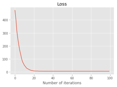
plt.plot(losses)
plt.title('Loss')
plt.xlabel('Number of iterations')
loss: 5.67: 100%|██████████| 100/100 [00:02<00:00, 44.90it/s]


Text(0.5,0,'Number of iterations')
Well, that’s it for this part. Stay tuned for the second part where we will build the transformer using the tools introduced here!