This is the second part of the analysis for the data from JH Dorrington Farm. You might want to read the first part before reading this one.
Before we put on our science hats, let us make an outline for what we will do. Previously we split the data into training and test sets 80/20. We will fit all of our models and calibrate them on the training set. Decisions about keeping/dropping predictors, transforming predictors and which model to chose will be left to the test set. Since we won’t have too many predictors (we will only use Age, Sire ID and milk based measurements), we can use 10 fold cross validation to decide on model parameters.
Next on to the topic of models.

Not those kind of models. OK, anyway, since my friend Chris probably wants to use the model to explain to him the relationship between milk related measurements and average calving intensity, we are going to stick to models that are interpretable. I’m sorry to disappoint those who were waiting for me to run a deep neural network on 1200 data points.
training.df = read_csv("../../data/jh-dorrington/train.csv")
test.df = read_csv("../../data/jh-dorrington/test.csv")

models = tribble(
  ~name, ~method,
  "Linear regression", "lm",
  "Robust LM", "rlm",
  "Slab & Spike regression", "spikeslab",
  "MARS", "earth",
  "CART", "rpart",
  "Elastic net", "enet",
  "Paritial least squares", "pls"
)
models %>%
table_print()| name | method |
|---|---|
| Linear regression | lm |
| Robust LM | rlm |
| Slab & Spike regression | spikeslab |
| MARS | earth |
| CART | rpart |
| Elastic net | enet |
| Paritial least squares | pls |
So those are our models. At this point, feel free to look them up if you don’t already know them.
Now we take all the milk based predictors, age and the response (average calving interval).
# Keep only the milk based predictors, Age and Average_calving_interval
milk.ind = c()
for(key in c("milk",
             "fat",
             "lac",
             "prot",
             "Age",
             "Average_calving_interval")){
  milk.ind = c(grep(paste0("*", key, "*"), names(training.df)), milk.ind)
}
milk.ind = unique(milk.ind)
milk.names = names(training.df)[milk.ind]
milk.names %>% print
#> [1] "Average_calving_interval" "Age"
#> [3] "Age_at_first_calving" "Life_prot_cfherd"
#> [5] "Lac_prot_kg" "D360_prot_kg"
#> [7] "Lac_prot_cfherd" "Mean_prot_perc"
#> [9] "Mean_lact_milk" "Mean_lac_perc"
#> [11] "Dam_lact_yield" "Life_fat_cfherd"
#> [13] "Lac_fat_kg" "D360_fat_kg"
#> [15] "Lac_fat_cfherd" "Mean_fat_perc"
#> [17] "Mean_305d_milk" "Life_milk_cfherd"
#> [19] "Lac_milk_kg" "D360_milk_kg"
#> [21] "Lac_milk_cfherd" "Life_milk_day"
#> [23] "Life_milk_recs"training.df = training.df %>%
dplyr::select(one_of(milk.names))
test.df = test.df %>%
dplyr::select(one_of(milk.names))
training.df %>% mutate(set = "Training") %>%
rbind(test.df %>% mutate(set = "Test")) %>%
group_by(set) %>%
summarise_all(funs(sum(is.na(.)))) %>%
gather(column, missing, -set) %>%
filter(missing > 0) %>%
ggplot(aes(reorder(column, missing), missing, fill = column)) +
geom_bar(stat = "identity") +
coord_flip() +
guides(fill = F) +
labs(
title = "Missing entries",
x = "",
y = "Number of missing entries"
) +
facet_wrap(~set)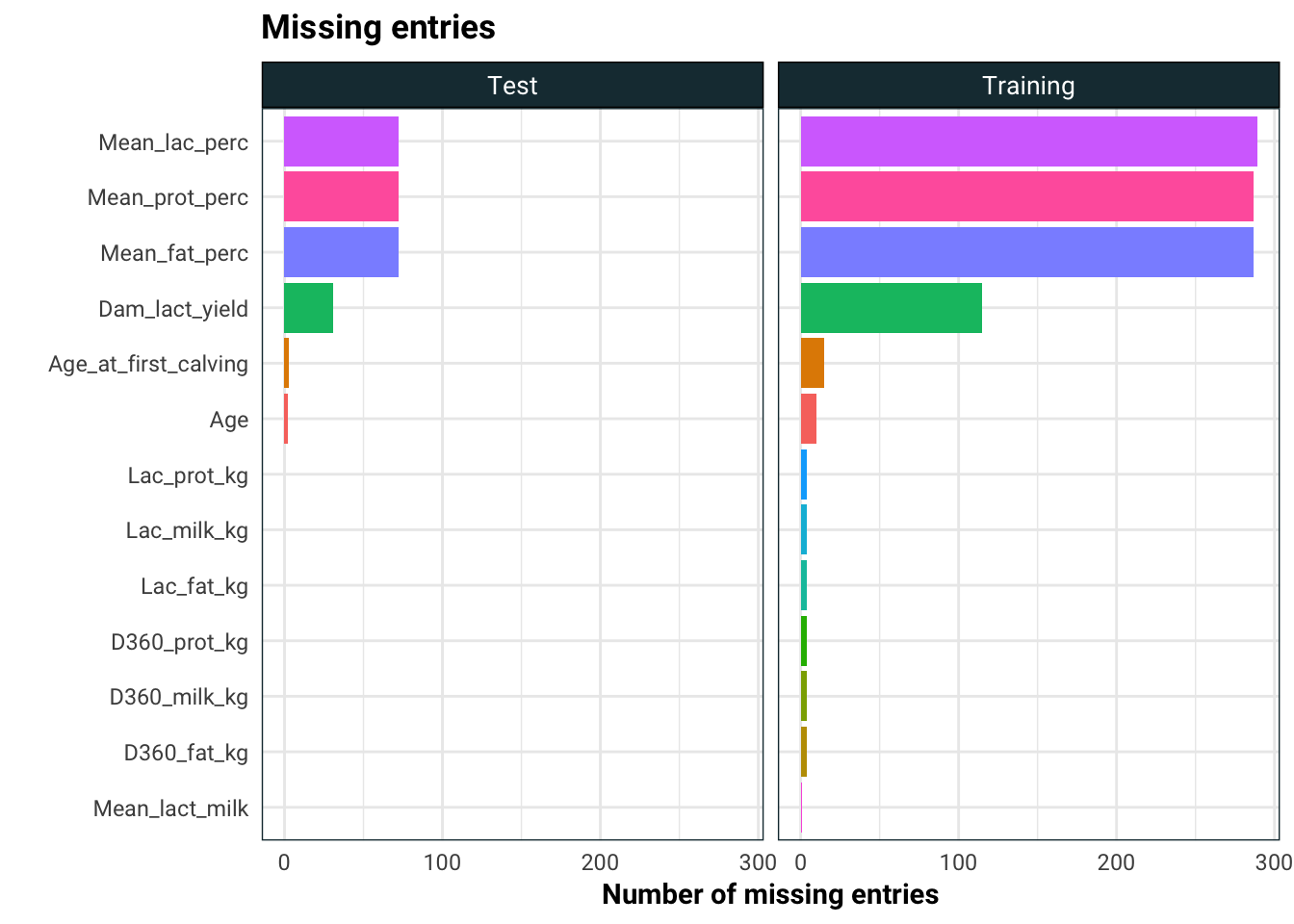
As we can see, there are quite a few entries missing. We are going to employ three strategies to deal with the missing entries:
- Drop the columns with large number of missing entries
- Fill the missing entries with 0.01 (this for CART, won’t work well on regression models)
- Fill the missing entries using the median
- Fill the missing entries using K nearest neighbour
We will see on the test set which of the three works the best.
How are we going to keep a track of all of this? We will make a data table which contains every possible choice we have made, an up to date training and test set depending on the choices and a fitted model.
library(caret)
library(RANN)
knn = preProcess(training.df, method = "knnImpute")
med = preProcess(training.df, method = "medianImpute")
fill_med = function(df){
  ret = predict(med, df)
  ret[1] = df[1]
  ret
}
fill_knn = function(df){
  ret = predict(knn, df)
  ret[1] = df[1]
  ret
}
drops = c("Mean_lac_perc",
    "Mean_prot_perc",
    "Mean_fat_perc",
    "Dam_lact_yield")
pre_data = tribble(
  ~fill_type, ~fill_parser,
  "Remove NA ", function(df) df %>% dplyr::select(-one_of(drops)) %>% drop_na,
  "Fill zero ", function(df) replace(df, is.na(df), 0.01),
  "Fill median ", fill_med,
  "Fill kNN ", fill_knn
) %>%
  mutate(training = map(fill_parser, function(f) f(training.df)),
         test = map(fill_parser, function(f) f(test.df))) %>%
  dplyr::select(-fill_parser)
pre_data %>%
  mutate(training = map(training, function(df) dim(df)),
         test = map(test, function(df) dim(df))) %>%
table_print()| fill_type | training | test |
|---|---|---|
| Remove NA | 999, 19 | 249, 19 |
| Fill zero | 1019, 23 | 252, 23 |
| Fill median | 1019, 23 | 252, 23 |
| Fill kNN | 1019, 23 | 252, 23 |
Next we make two adjustments to the data set, one where we drop one of correlated variables where we set the cut-off at .75.
drops.cor = findCorrelation(cor(training.df[-1] %>% drop_na),
                           cutoff = .75,
                           names = T)
drop_cor = function(type, df){
  if(type != "rm cor") return(df)
  df %>%
    dplyr::select(-one_of(drops.cor))
}
pre_data = pre_data %>%
  merge(tibble(cor_drop = c("", "rm cor"))) %>%
  mutate(training = map2(cor_drop, training, drop_cor),
         test = map2(cor_drop, test, drop_cor))
After this choice, we have yet an other two choices. Since our predictors are all positive, we can chose to apply a Box-Cox transformation if we so chose. Incidently, I stumbled on this bug. In short, Box-Cox does not play well with tibble.
When we are doing this, we have to be careful. We have already manipulated the training data before. So for each
box_cox_fun = function(df){
  preProcess(df %>% as.data.frame,
             method = "BoxCox")
}

apply_bc = function(bc, df){
  ret = predict(bc, df %>% as.data.frame)
  ret[1] = df[1]
  ret %>% as.tibble
}

pre_data = pre_data %>%
  mutate(box_cox_fun = map(training, box_cox_fun),
         box_cox = " Box-Cox",
         training = map2(box_cox_fun, training, apply_bc),
         test = map2(box_cox_fun, test, apply_bc)) %>%
  dplyr::select(-box_cox_fun) %>%
  rbind(pre_data %>% mutate(box_cox = "")) %>%
  mutate(transform = paste0(fill_type, cor_drop, box_cox)) %>%
  dplyr::select(transform, training, test) %>%
  as.tibble
pre_data %>%
  mutate(training = map(training, function(df) dim(df)),
         test = map(test, function(df) dim(df))) %>%
table_print()| transform | training | test |
|---|---|---|
| Remove NA Box-Cox | 999, 19 | 249, 19 |
| Fill zero Box-Cox | 1019, 23 | 252, 23 |
| Fill median Box-Cox | 1019, 23 | 252, 23 |
| Fill kNN Box-Cox | 1019, 23 | 252, 23 |
| Remove NA rm cor Box-Cox | 999, 8 | 249, 8 |
| Fill zero rm cor Box-Cox | 1019, 12 | 252, 12 |
| Fill median rm cor Box-Cox | 1019, 12 | 252, 12 |
| Fill kNN rm cor Box-Cox | 1019, 12 | 252, 12 |
| Remove NA | 999, 19 | 249, 19 |
| Fill zero | 1019, 23 | 252, 23 |
| Fill median | 1019, 23 | 252, 23 |
| Fill kNN | 1019, 23 | 252, 23 |
| Remove NA rm cor | 999, 8 | 249, 8 |
| Fill zero rm cor | 1019, 12 | 252, 12 |
| Fill median rm cor | 1019, 12 | 252, 12 |
| Fill kNN rm cor | 1019, 12 | 252, 12 |
That’s all the choices bundled into one data structure. Just as a side note, R is pretty smart about retaining memory for duplicated structures, so pre_data object above is not actually taking up too much memory.
Now for each choice we made pre-processing the data, we add on the choice of model. Then we fit each model + pre-processing combo where we run 10-fold cross validation to select the parameters. By default, caret will perform a grid search with a predefined grid, which is good enough for us.
library(foreach)
trControl = trainControl(method = "cv",
                         number = 10)
fit_model = function(method, df){
  train(Average_calving_interval ~ .,
        data = df,
        trControl = trControl,
        method = method)
}
models = merge(models, pre_data) %>%
  as.tibble %>%
  mutate(fit = map2(method, training, fit_model))
Now we can finally see the model performance.
eval_model = function(fit, df){
  preds = predict(fit, df[-1])
  (preds - df[1])^2 %>% mean %>% sqrt
}
models = models %>%
  mutate(rmse = map2_dbl(fit, test, eval_model)) %>%
  arrange(rmse)
models %>%
  ggplot(aes(rmse, name, colour = transform)) +
  geom_point(size = 2) +
  guides(colour = guide_legend(title = "Preprocess")) +
  labs(
    title = "Performance of the models on the test set",
    x = "RMSE",
    y = ""
  )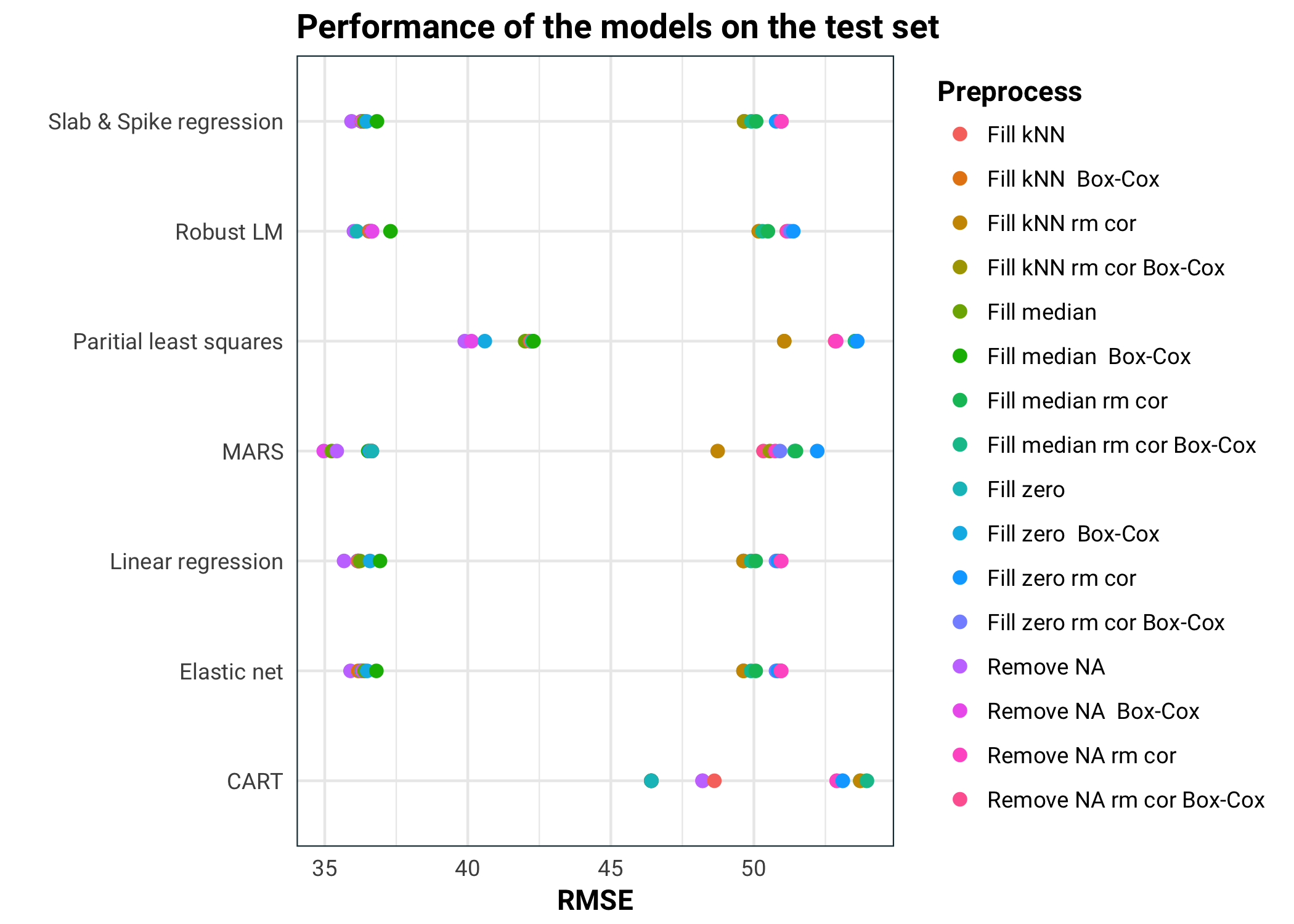
In conclusion, we can see that MARS performs the best. All the pure linear models perform about the same. Elastic net and spike & slab regressions also perform feature selection, so it will be interesting to see if they kept the same information. MARS performs better with the correlated predictors removed Partial least squares isn’t performing as well, probably because it kept too few of the components. Lastly we have CART, which did really badly. This is not surprising, since our data is pretty noisy, high bias models tend to outperform low bias ones.
Stay tuned for an other episode where we will pick apart the models and finally give some answers.